Water Conservation for Michigan – Why?

The Michigan Association of Planners joined several environmental groups to pass state legislation requiring water conservation for public, and private users.

Among the legislation are laws requiring low flush toilets, and prohibiting high-volume shower heads as in this Seinfeld episode. I suppose I should go along: I’m running for water commissioner, and consider myself a conservationist. The problem is, I can’t see a good argument for these laws here in Oakland County, or in neighboring Macomb and Wayne Counties. The water can’t run out because most users take it from the Detroit river and return it there, cleaned after it’s used; it’s all recycled.

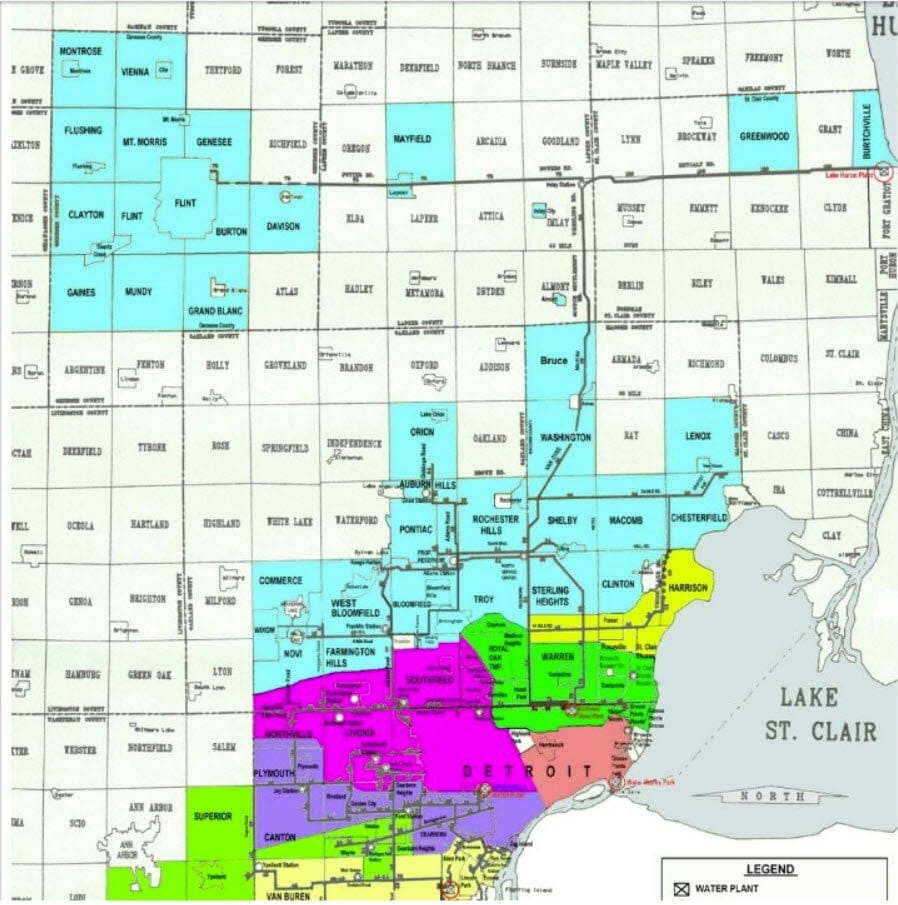
Map of the main drinking-water pipes serving south-east Michigan

Map of the main drinking-water pipes serving south-east Michigan

The map above shows the clean water system for south-east Michigan. The high-population areas, the ones that are colored in the map, get their water from the Detroit River or from Lake Huron. It’s cleaned, pumped, and carried to your home along the pipes shown. Then after you’ve used the water, it travels back along another set of pipes to the water treatment plant and into the Detroit River.

Three-position shower head -- a wonderful home improvement  I got it at universal plumbing.

Three-position shower head — a wonderful home improvement. I got it at universal plumbing.

When the system is working well, the water we return to the Detroit River is cleaner than the water we took in. So why legislate against personal use? If a customer wants to enjoy a good shower, and is willing to pay for the water at 1.5¢ per gallon, who cares how much water that customer uses? I can understand education efforts, sort-of, but find it hard to push legislation like we have against a high-volume shower head. We can not run out, and the more you use, the less everyone pays per gallon. A great shower head is a great gift idea, in my opinion.

The water department does not always work well, by the way, and these problems should be solved by legislation. We give away, for $200/year, high value clean water to Nestle company and then buy it back for $100,000,000. That’s a problem. Non-flushable toilet wipes are marketed as flushable; this causes sewer blockades. Our combined sewers regularly dump contaminated water into our rivers, lakes, and basements. These problems can be solved with legislation and engineering. It’s these problems that I’m running to solve.

Robert Buxbaum, January 6, 2019. If you want to save water, either to save the earth, or because you are cheep, here are some conservation ideas that make sense (to me).

The hard scrabble dictionary

The rules or Scrabble are unchanging and always changing. The general rule is that Scrabble allows the use of every common word in the English language. In practice, there are two or more dictionaries of words. One of these has virtually no abbreviations, only a few foreign-derived words, and only a select few offensive terms. It is this one, “The Official Scrabble Players Dictionary,” that determines play. You’ll need the other dictionary to look up swear words or secondary meanings, or find common abbreviations.

Words get removed from the scrabble dictionary when someone -- anyone might find them offensive.

Words get removed from the scrabble dictionary when someone — anyone might find them offensive.

Both of these dictionaries change on a regular basis, by the way. And this is as it should be, and both exist in both English and American versions. The common dictionary adds words slowly, as they come into use and drops them slowly as they fall out. The Scrabble dictionary changes fast and for no obvious reason, adding and removing words for political and social aspect and for improved playability (whatever that is). Thus there is little rhyme or reason to the additions or deletions. Four years ago some ten 4000 words were added, mostly unusual words, and many insult words were removed. When the dictionary was changed again in September of this year, players are not told of some changes, but for the most part, there no obvious way to guess. Several words that were offensive in the last version, now are not. Other words that were OK then are now removed as offensive. You’ll play a word you’ve used for years and be told that it is no longer valid. Or someone will use a word you’ve never seen, and never will see otherwise, and you’ll find it is valid. Words added this year include: OK (previously an abbreviation), zen (previously a foreign word), and sheeple (previously a portmanteau, non-word). Also, I’m happy to say, fuck (a welcome addition). I looked up a bunch of previously removed insult words, and find that goy and spic are back, but i find that negro is not.  There is no list in print that tells you what’s been added, and that’s not right. Some articles have a few examples of new words, and some claim to have a list, but clearly it’s only a small fraction of the real list. There is nothing like a full addition list that I could find.

I’ve a bigger gripe though against removed words, especially when they are common words made to disappear for political effect. The previous dictionary, 2014, removed spic, goy, goyim, and negro; that was not right. The current dictionary added back all but negro (check for yourself, here). The word is still in use, both verbally and in literature, and not particularly offensive, less offensive than spic, IMHO. The American Negro College Fund doesn’t seem to mind the word negro. Malcolm X didn’t either. No one tells you these words are gone; they just disappear in the night.

My opinion, such as it is. I’m asking Mattel, Hasbro, Colliers, and/or Merriam-Webster: allow in all normal words, despite the fact that several have implied insults, or real ones. AND PUBLISH A COMPLETE CORRECTIONS PAGE, you [non recognized word]. Thank you.

Robert Buxbaum, December 27, 2018.

We don’t need no stinking primary clarifier

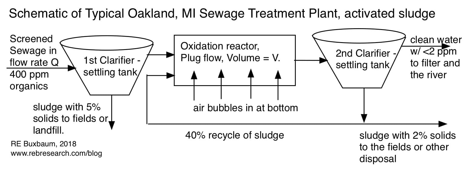
Virtually every sewage plant of Oakland County uses the activated sludge process, shown in the layout below. Raw sewage comes in, and goes through physical separation — screening, grit removal, and a first clarifier – settling tank before moving to the activated sludge oxidation reactor. The 1st clarifier, shown at left below, removes about half of the incoming organics, but it often stinks and sometimes it “pops” bubbles of fart. This is usually during periods of low flow, like at night. When the flow is slow, it arrives at the plant as a rotting smelly mess; it’s often hard to keep the bubbles of smell down.

Typical Oakland Sewage plant, activated sludge process with a primary clarifier.

Typical Oakland County Sewage treatment plant, activated sludge process with a primary clarifier.

The smell is much improved in the oxidation reactor, analyzed here, and in the 2nd clarifier, shown above at right. Following that is a filter, an ultraviolet cleanup stage, and the liquids are discharged to a local river. In Oakland county, the solids from the two clarifiers are hauled off to a farm, or buried in a landfill. Burial in a landfill is a costly waste, as I discuss here. The throughputs for most of these treatment plants is only about 2-3 million gallons of sewage per day. But Oakland county can produce 500 million gallons of sewage per day. The majority of this goes to Detroit for treatment, and sometimes the overflow is dumped rotting and smelly, in the rivers.

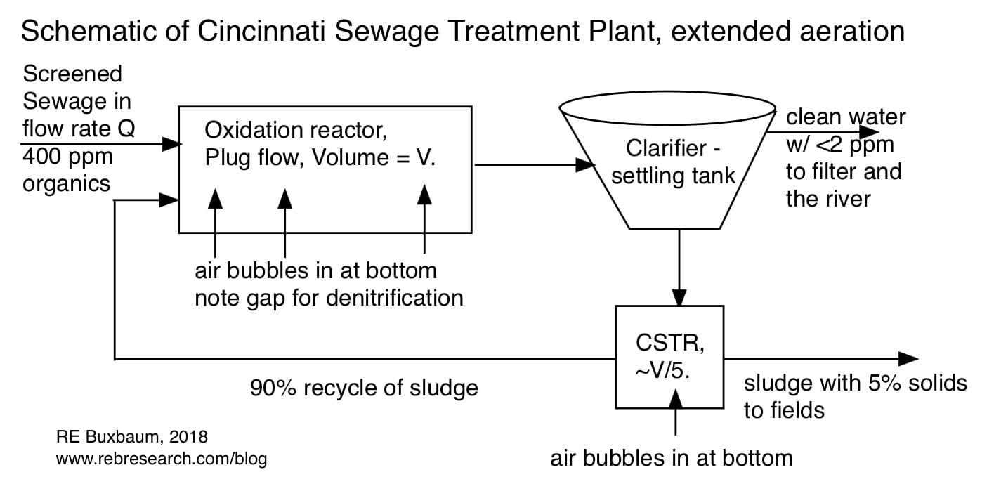
A few months ago, I visited the Sycamore Creek Wastewater facility outside of Cincinnati. This is an 8 million gallon per day plant that uses the “extended aeration process”, shown in the sketch below. I noticed several things I liked: the high throughput (the plant looks no bigger than our 2-3 million gallon plants) and the lack of a bad smell, primarily. The Sycamore Creek plant had an empty hole where the primary clarifier had once been. Lacking this clarifier, the screened sewage could not sit and pop. Instead it goes directly from grit removal to the oxidation reactor, a reactor that looks no bigger than in our plants. This reactor manages a four times higher throughput, I think, because of a higher concentration of cellular catalyst. Consider the following equation derived in a previous post:

ln C°/C = kV/Q.

Here, C° and C are the incoming and exit concentrations of soluble organic; k is the reaction rate, proportional to cellular concentration, V is the volume of the reactor, Q is the flow, and ln is natural log. The higher cellular concentration in the extended aeration plant results in an increased reaction rate, k. The higher the value of k, the higher the allowed flow, Q, per reactor volume, V.

The single clarifier at the end of the Sycamore Creek plant does not look particularly big. My sense is that it deals with a lot more sludge and flow than is seen in our 2nd clarifiers because (I imaging) the sludge is higher density, thus faster settling. I expect that, without the 1 clarifier, there is extra iron and sulfate in the sludge, and more large particles too. In our plants, a lot of these things are removed in the primary clarifier. Sludge density is also increased, I think, because the Cincinnati plant recycle a greater percentage of the sludge (I list it as 90% in the diagram). Extra iron in the reactor also helps to remove phosphates from the water effluent that flows back to the river, an important pollution concern. Iron phosphates are insoluble, and thus leave with the sludge. In Oakland county’s activated sludge plants, it is typical to add iron to the reactor or clarifier. In Cincinnati’s extended aeration plant, I’m told, iron addition is generally not needed.

Typical Oakland Sewage plant, activated sludge process with a primary clarifier.

Cincinnati sewage treatment plant, extended aeration process with no primary clarifier.

The extended aeration part of the above process refers to the secondary sludge oxidizer, the continuously stirred tank reactor, or CSTR shown at lower right above. The “CSTR” is about 1/5 the volume of the main oxidation reactor and about the size of a clarifier. Oxidation in the CSTR compliments that in the main oxidizer removing organics, making bio-polymer, and improving (I think) the quality of the sludge that goes to the farms. Oxidation in the CSTR reduces the amount of sludge that goes to the farms. The sludge that does go, is  less-toxic and more concentrated in organics and minerals. I’m not sure if the CSTR product is as good as the product from an anaerobic digester, or if the CSTR is cheaper to operate, but it looks cheaper since there is no roof, and no (or minimal) heating. This secondary oxidizer is very efficient at removing organics because the cellular catalyst concentration is very high – much higher than in the main oxidizer.

During periods of high load, early morning, the CSTR seems to serve as a holding tank so that sludge does not build up in the clarifier. Too much sludge in the clarifier can start to rot, and ruin the effluent quality. The way you tell if there is too much sludge, by the way, is through a device called the “sludge judge.” I love that name. The Cincinnati plant used a centrifugal drier; none of our plants do. The Cincinnati plant had gap the bubble spots of the main oxidizer. This is good for denitrification, I’m told, an important process that I discuss elsewhere.

The liquid output of their clarifier (or ours) is not pure enough to be sent directly to the river. In this plant, the near-pure water from the clarifier is sent to a trickling filter, a bed of sand and anthracite that removes colloidal remnants. Some of our plants do the same. I suspect that the large surface area in this filter is also home to some catalysis: last stage oxidation of remaining bio-organics. On a regular basis, the filter bed is reverse-flushed to remove cellular buildup, slime, and send it to the beginning of the process. The trickling filter output is then sent to an ultraviolet, bacteria-killing step before being released to the rivers. All in all, I suspect that an extended aeration process like this is worth looking into for Oakland County, especially for our North Pontiac sewage treatment facility. That plant is particularly bad smelling, and clearly too small to treat all its sewage. Perhaps we can increase the throughput and decrease the smell at a minimal cost.

Dr. Robert E. Buxbaum, December 18, 2018. I’m running for water commissioner of Oakland county, MI. If you like, visit my campaign site. Here are some sludge jokes and my campaign song.

Measles, anti-vaxers, and the pious lies of the CDC.

Measles is a horrible disease that contributed to the downfall that had been declared dead in the US, wiped out by immunization, but it has reappeared. A lot of the blame goes to folks who refuse to vaccinate: anti-vaxers in the popular press. The Center for Disease Control is doing its best to promote to stop the anti-vaxers, and promote vaccination for all, but in doing so, I find they present the risks of measles worse than they are. While I’m sympathetic to the goal, I’m not a fan of bending the truth. Lies hurt the people who speak them and the ones who believe them, and they can hurt the health of immune-compromized children who are pushed to vaccinate. You will see my arguments below.

The CDC’s most-used value for the mortality rate for measles is 0.3%. It appears, for example, in line two of the following table from Orenstein et al., 2004. This table also includes measles-caused complications, broken down by type and patient age; read the full article here.

Measles complications, death rates, US, 1987-2000, CDC.

Measles complications, death rates, US, 1987-2000, CDC, Orenstein et. al. 2004.

The 0.3% average mortality rate seems more in tune with the 1800s than today. Similarly, note that the risk of measles-associated encephalitis is given as 10.1%, higher than the risk of measles-diarrhea, 8.2%. Do 10.1% of measles cases today produce encephalitis, a horrible, brain-swelling disease that often causes death. Basically everyone in the 1950s and early 60s got measles (I got it twice), but there were only 1000 cases of encephalitis per year. None of my classmates got encephalitis, and none died. How is this possible; it was the era before antibiotics. Even Orenstein et. al comment that their measles mortality rates appear to be far higher today than in the 1940s and 50s. The article explains that the increase to 3 per thousand, “is most likely due to more complete reporting of measles as a cause of death, HIV infections, and a higher proportion of cases among preschool-aged children and adults.”

A far more likely explanation is that the CDC value is wrong. That the measles cases that were reported and certified as such are the ones that are the most severe. There were about 450 measles deaths per year in the 1940s and 1950s, and 408 in 1962, the last year before the MMR vaccine was developed and by Dr. Hilleman of Merck (a great man of science, forgotten). In the last two decades there were some 2000 measles cases reported US cases but only one measles death. A significant decline in cases, but the ratio does not support the CDC’s death rate. For a better estimate, I propose to divide the total number of measles deaths in 1962 by the average birth rate in the late 1950s. That is to say, I propose to divide 408 by the 4.3 million births per year. From this, I calculate a mortality rate just under 0.01% in 1962, That’s 1/30th the CDC number, and medicine has improved since 1962.

I suspect that the CDC inflates the mortality numbers, in part by cherry-picking its years. It inflates them further by treating “reported measles cases.” as if they were all measles cases. I suspect that the reported cases in these years were mainly the very severe ones. Mild case measles clears up before being reported or certified as measles. This seems the only normal explanation for why 10.1% of cases include encephalitis, and only 8.2% diarrhea. It’s why the CDC’s mortality numbers suggest that, despite antibiotics, our death rate has gone up by a factor of 30 since 1962.

Consider the experience of people who lived in the early 60s. Most children of my era went to public elementary schools with some 1000 other students, all of whom got measles. By the CDC’s mortality number, we should have seen three measles deaths per school, and 101 cases of encephalitis. In reality, if there had been one death in my school it would have been big news, and it’s impossible that 10% of my classmates got encephalitis. Instead, in those years, only 48,000 people were hospitalized per year for measles, and 1,000 of these suffered encephalitis (CDC numbers, reported here).

To see if vaccination is a good idea, lets now consider the risk of vaccination. The CDC reports their vaccine “is virtually risk free”, but what does risk-free mean? A British study finds vaccination-caused neurological damage in 1/365,000 MMR vaccinations, a rate of 0.00027%, with a small fraction leading to death. These problems are mostly found in immunocompromised patients. I will now estimate the neurological risk for actual measles based on the ratio of encephalitis to births, as before using the average birth rate as my estimate for measles cases; 1000/4,300,000 = 0.023%. This is far lower than the risk the CDC reports, and more in line with experience.

The risk for neurological damage from measles that I calculate is 86 times higher risk than the neurological risk from vaccination, suggesting vaccination is a very good thing, on average: The vast majority of people should get vaccinated. But for people with a weakened immune system, my calculations suggest it is worthwhile to not immunize at 12 months as doctors recommend. The main cause of vaccination death is encephalitis, but this only happens in patients with weakened immune systems. If your child’s immune system is weakened, even by a cold, I’d suggest you wait 1-3 months, and would hope that your doctor would concur. If your child has AIDS, ALS, Lupus, or any other, long-term immune problem, you should not vaccinate at all. Not vaccinating your immune-weakened child will weaken the herd immunity, but will protect your child.

We live in a country with significant herd immunity: Even if there were a measles outbreak, it is unlikely there would be 500 cases at one time, and your child’s chance of running into one of them in the next month is very small assuming that you don’t take your child to Disneyland, or to visit relatives from abroad. Also, don’t hang out with anti-vaxers if you are not vaccinated. Associating with anti-vaxers will dramatically increase your child’s risk of infection.

As for autism: there appears to be no autism advantage to pushing off vaccination. Signs of autism typically appear around 12 months, the same age that most children receive their first-stage MMR shot, so some people came to associate the two. Parents who push-off vaccination do not push-off the child’s chance of developing autism, they just increase the chance their child will get measles, and that their child will infect others. Schools are right to bar such children, IMHO.

I’ve noticed that, with health care in, particular, there is a tendency for researchers to mangle statistics so that good things seem better than they are. Health food: is not necessarily so healthy as they say; nor is weight lossBicycle helmets: ditto. Sometimes this bleeds over to outright lies. Generic modified grains were branded as cancer-causing based on outright lies and  missionary zeal. I feel that I help a bit, in part by countering individual white lies; in part by teaching folks how to better read statistic arguments. If you are a researcher, I strongly suggest you do not set up your research with a hypothesis so that only one outcome will be publishable or acceptable. Here’s how.

Robert E. Buxbaum, December 9, 2018.

China worse than the US in CO2 per output

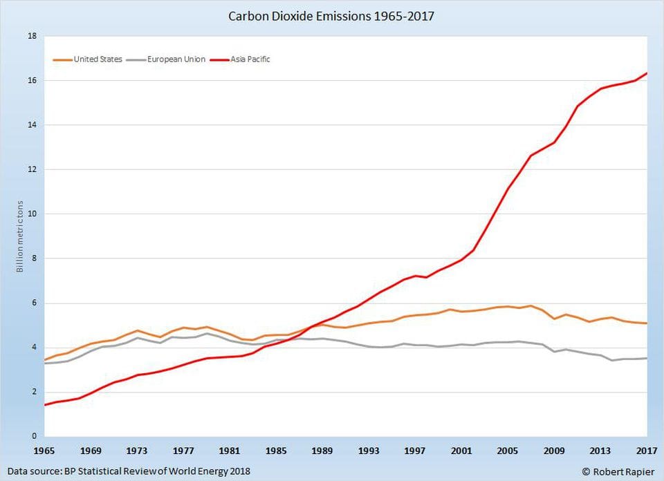
CO2 per year, 1965-2017, China and developed world

CO2 output per year, 1965-2017, China and developed world

For the last decade at least, China has been the industrial  manufacturer to the world. If not for Chinese shoes, the US would go barefoot. if not for Chinese electronics, Americans would be without iPhones, laptops, and TVs. China still trails the US and Europe in banking, software, movies and the like, but relying on China for manufactured goods is a dangerous position for the free world economically, and it’s not much better in terms of pollution.

China is among the world’s worst polluters. It burns coal for power to an extent that the air quality of China’s major cities would be unacceptable most everywhere else. On most days, it is thick with a yellow and grey haze. By 1969 China had passed the US and the European union in terms of CO2 production. And, as 2017, they produce nearly three times as much CO2 as the USA, four times more than the entire European Union. While China claims an interest in changing, the amount of pollution China’s CO2 output is still growing while ours and the EU’s is decreasing.

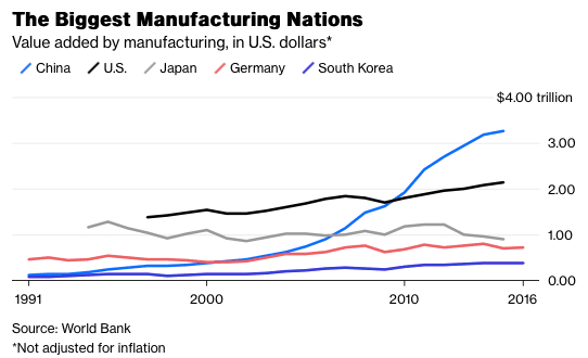
Manufacturing in the US, China, EU, Japan, Korea. Source: World Bank.

Manufacturing in the US, China, Germany, Japan, Korea. Source: World Bank.

China’s pollution would not be so bad if it were an efficient manufacturer, but there is a lot to suggest that it is not. China produces 50% more industrial goods than the US, but employs far more man hours, and generates more than three times the  CO2. Even in a fairly developed industry like steel, the US uses fewer man hours per ton and generates less CO2. I’m thus drawn to conclude that US companies off-load work to China mainly to get around US labor and pollution laws. Alternately, they off-load manufacture to gain entry to the Chinese market, a market that is otherwise closed to them. When US companies do this, they benefit the corporate managers and owners, but not the US worker. 

The hope (expectation) is that president Trump’s tariffs on Chinese goods will decrease the wage advantage of manufacturing in China, and will decrease the amount of US goods manufactured there. Some of that production, I expect, will move to the US, some will remain in China, and will be imported at a higher price-point. I expect a net decrease in CO2 as the US appears to be the more efficient producer, and because fewer ships will be crossing the Pacific bringing Chinese goods to the US. I expect some increase in tax revenue to the US, and some price inflation as well, as importers pass along the increased cost of Chinese goods. Overall, I think this is an acceptable trade-off, but what do I know.

Robert Buxbaum, November 29, 2018

A logic joke, and an engineering joke.

The following is an oldish logic joke. I used it to explain a conclusion I’d come to, and I got just a blank stare and a confused giggle, so here goes:

Three logicians walk into a bar. The barman asks: “Do all of you want the daily special?” The first logician says, “I don’t know.” The second says, “I don’t know.” The third says, “yes.”

The point of the joke was that, in several situations, depending on who you ask, “I don’t know” can be a very meaningful answer. Similarly, “I’m not sure.”  While I’m at it, here’s an engineering education joke, it’s based on the same logic, here applied:

A team of student engineers builds an airplane and wheel it out before the faculty. “We’ve designed this plane”, they explain, “based on the principles and methods you taught us. “We’ve checked our calculations rigorously, and we’re sure we’ve missed nothing. “Now. it would be a great honor to us if you would join us on its maiden flight.”

At this point, some of the professors turn white, and all of them provide various excuses for why they can’t go just now. But there is one exception, the dean of engineering smiles broadly, compliments the students, and says he’ll be happy to fly. He gets onboard the plane seating himself in the front of the plane, right behind the pilot. After strapping himself in, a reporter from the student paper comes along and asks why he alone is willing to take this ride; “Why you and no one else?” The engineering dean explains, “You see, son, I have an advantage over the other professors: Not only did I teach many of you, fine students, but I taught many of them as well.” “I know this plane is safe: There is no way it will leave the ground.”heredity cartoon

Robert Buxbaum, November 2i, 2018.  And one last. I used to teach at Michigan State University. They are fine students.

James Croll, janitor scientist; man didn’t cause warming or ice age

When politicians say that 98% of published scientists agree that man is the cause of global warming you may wonder who the other scientists are. It’s been known at least since the mid 1800s that the world was getting warmer; that came up talking about the president’s “Resolute” desk, and the assumption was that the cause was coal. The first scientist to present an alternate theory was James Croll, a scientist who learned algebra only at 22, and got to mix with high-level scientists as the janitor at the Anderson College in Glasgow. I think he is probably right, though he got some details wrong, in my opinion.

James Croll was born in 1821 to a poor farming family in Scotland. He had an intense interest in science, but no opportunity for higher schooling. Instead he worked on the farm and at various jobs that allowed him to read, but he lacked a mathematics background and had no one to discuss science with. To learn formal algebra, he sat in the back of a class of younger students. Things would have pretty well ended there but he got a job as janitor for the Anderson College (Scotland), and had access to the library. As janitor, he could read journals, he could talk to scientists, and he came up with a theory of climate change that got a lot of novel things right. His idea was that there were  regular ice ages and warming periods that would follow in cycles. In his view these were a product of the precession of the equinox and the fact that the earth’s orbit was not round, but elliptical, with an eccentricity of 1.7%. We are 3.4% closer to the sun on January 3 than we are on July 4, but the precise dates changes slowly because of precession of the earth’s axis, otherwise known as precession of the equinox.

Currently, at the spring equinox, the sun is in “the house of Pisces“. This is to say, that a person who looks at the stars all the night of the spring equinox will be able to see all of the constellations of the zodiac except for the stars that represent Pisces (two fish). But the earth’s axes turns slowly, about 1 days worth of turn every 70 years, one rotation every 25,770 years. Some 1800 years ago, the sun would have been in the house of Ares, and 300 years from now, we will be “in the age of Aquarius.” In case you wondered what the song, “age of Aquarius” was about, it’s about the precession of the equinox.

Our current spot in the precession, according to Croll is favorable to warmth. Because we are close to the sun on January 3, our northern summers are less-warm than they would be otherwise, but longer; in the southern hemisphere summers are warmer but shorter (southern winters are short because of conservation of angular momentum). The net result, according to Croll should be a loss of ice at both poles, and slow warming of the earth. Cooling occurs, according to Croll, when the earth’s axis tilt is 90° off the major axis of the orbit ellipse, 6300 years before or after today. Similar to this, a decrease in the tilt of the earth would cause an ice age (see here for why). Earth tilt varies over a 42,000 year cycle, and it is now in the middle of a decrease. Croll’s argument is that it takes a real summer to melt the ice at the poles; if you don’t have much of a tilt, or if the tilt is at the wrong time, ice builds making the earth more reflective, and thus a little colder and iceier each year; ice extends south of Paris and Boston. Eventually precession and tilt reverses the cooling, producing alternating warm periods and ice ages. We are currently in a warm period.

Global temperatures measured from the antarctic ice showing stable, cyclic chaos and self-similarity.

Global temperatures measured from the antarctic ice showing stable, cyclic chaos and self-similarity.

At the time Croll was coming up with this, it looked like numerology. Besides, most scientists doubted that ice ages happened in any regular pattern. We now know that ice ages do happen periodically and think that Croll must have been on to something. See figure; the earth’s temperature shows both a 42,000 year cycle and a 23,000 year cycle with ice ages coming every 100,000 years.

In the 1920s a Serbian Mathematician, geologist, astronomer, Milutin Milanković   proposed a new version of Croll’s theory that justified longer space between ice ages based on the beat frequency between a 23,000 year time for axis precession, and the 42,000 year time for axis tilt variation. Milanković used this revised precession time because the ellipse precesses, and thus the weather-related precession of the axis is 23,000 years instead of 25,770 years. The beat frequency is found as follows:

51,000 = 23,000 x 42,000 / (42000-23000).

As it happens neither Croll’s nor Milanković’s was accepted in their own lifetimes. Despite mounting evidence that there were regular ice ages, it was hard to believe that these small causes could produce such large effects. Then, in a 1976 study (Hayes, Imbrie, and Shackleton) demonstrated clear climate variations based on the mud composition from New York and Arizona. The variations followed all four of the Milankocitch cycles.

Southern hemisphere ice is growing, something that confounds CO2-centric experts

Southern hemisphere ice is growing, something that confounds CO2-centric experts

Further confirmation came from studying the antarctic ice, above. You can clearly see the 23,000 year cycle of precession, the 41,000 year cycle of tilt, the 51,000 year beat cycle, and also a 100,000 year cycle that appears to correspond to 100,000 year changes in the degree of elliptic-ness of the orbit. Our orbit goes from near circular to quite elliptic (6.8%) with a cycle time effectively of 100,000 years. It is currently 1.7% elliptic and decreasing fast. This, along with the decrease in earth tilt suggests that we are soon heading to an ice age. According to Croll, a highly eccentric orbit leads to warming because the minor access of the ellipse is reduced when the orbit is lengthened. We are now heading to a less-eccentric orbit; for more details go here; also for why the orbit changes and why there is precession.

We are currently near the end of a 7,000 year warm period. The one major thing that keeps maintaining this period seems to be that our precession is such that we are closest to the sun at nearly the winter solstice. In a few thousand years all the factors should point towards global cooling, and we should begin to see the glaciers advance. Already the antarctic ice is advancing year after year. We may come to appreciate the CO2 produced by cows and Chinese coal-burning as these may be all that hold off the coming ice age.

Robert Buxbaum, November 16, 2018.

Of God and gauge blocks

Most scientists are religious on some level. There’s clear evidence for a big bang, and thus for a God-of-Creation. But the creation event is so distant and huge that no personal God is implied. I’d like to suggest that the God of creation is close by and as a beginning to this, I’d like to discus Johansson gauge blocks, the standard tool used to measure machine parts accurately.

jo4

A pair of Johansson blocks supporting 100 kg in a 1917 demonstration. This is 33 times atmospheric pressure, about 470 psi.

Lets say you’re making a complicated piece of commercial machinery, a car engine for example. Generally you’ll need to make many parts in several different shops using several different machines. If you want to be sure the parts will fit together, a representative number of each part must be checked for dimensional accuracy in several places. An accuracy requirement of 0.01 mm is not uncommon. How would you do this? The way it’s been done, at least since the days of Henry Ford, is to mount the parts to a flat surface and use a feeler gauge to compare the heights of the parts to the height of stacks of precisely manufactured gauge blocks. Called Johansson gauge blocks after the inventor and original manufacturer, Henrik Johansson, the blocks are typically made of steel, 1.35″ wide by .35″ thick (0.47 in2 surface), and of various heights. Different height blocks can be stacked to produce any desired height in multiples of 0.01 mm. To give accuracy to the measurements, the blocks must be manufactured flat to within 1/10000 of a millimeter. This is 0.1µ, or about 1/5 the wavelength of visible light. At this degree of flatness an amazing thing is seen to happen: Jo blocks stick together when stacked with a force of 100 kg (220 pounds) or more, an effect called, “wringing.” See picture at right from a 1917 advertising demonstration.

This 220 lbs of force measured in the picture suggests an invisible pressure of 470 psi at least that holds the blocks together (220 lbs/0.47 in2 = 470 psi). This is 32 times the pressure of the atmosphere. It is independent of air, or temperature, or the metal used to make the blocks. Since pressure times volume equals energy, and this pressure can be thought of as a vacuum energy density arising “out of the nothingness.” We find that each cubic foot of space between the blocks contains, 470 foot-lbs of energy. This is the equivalent of 0.9 kWh per cubic meter, energy you can not see, but you can feel. That is a lot of energy in the nothingness, but the energy (and the pressure) get larger the flatter you make the surfaces, or the closer together you bring them together. This is an odd observation since, generally get more dense the smaller you divide them. Clean metal surfaces that are flat enough will weld together without the need for heat, a trick we have used in the manufacture of purifiers.

A standard way to think of quantum scattering is that the particle is scattered by invisible bits of light (virtual photons), the wavy lines. In this view, the force that pushes two flat surfaces together is from a slight deficiency in the amount of invisible light in the small space between them.

A standard way to think of quantum scattering of an atom (solid line) is that it is scattered by invisible bits of light, virtual photons (the wavy lines). In this view, the force that pushes two blocks together comes from a slight deficiency in the number of virtual photons in the small space between the blocks.

The empty space between two flat surfaces also has the power to scatter light or atoms that pass between them. This scattering is seen even in vacuum at zero degrees Kelvin, absolute zero. Somehow the light or atoms picks up energy, “out of the nothingness,” and shoots up or down. It’s a “quantum effect,” and after a while physics students forget how odd it is for energy to come out of nothing. Not only do students stop wondering about where the energy comes from, they stop wondering why it is that the scattering energy gets bigger the closer you bring the surfaces. With Johansson block sticking and with quantum scattering, the energy density gets higher the closer the surface, and this is accepted as normal, just Heisenberg’s uncertainly in two contexts. You can calculate the force from the zero-point energy of vacuum, but you must add a relativistic wrinkle: the distance between two surfaces shrinks the faster you move according to relativity, but measurable force should not. A calculation of the force that includes both quantum mechanics and relativity was derived by Hendrik Casimir:

Energy per volume = P = F/A = πhc/ 480 L4,

where P is pressure, F is force, A is area, h is plank’s quantum constant, 6.63×10⁻³⁴ Js, c is the speed of light, 3×10⁸ m/s, and L is the distance between the plates, m. Experiments have been found to match the above prediction to within 2%, experimental error, but the energy density this implies is huge, especially when L is small, the equation must apply down to plank lengths, 1.6×10⁻³⁵ m. Even at the size of an atom, 1×10⁻¹⁰m, the amount of the energy you can see is 3.6 GWhr/m3, 3.6 Giga Watts. 3.6 GigaWatt hrs is one hour’s energy output of three to four large nuclear plants. We see only a tiny portion of the Plank-length vacuum energy when we stick Johansson gauge blocks together, but the rest is there, near invisible, in every bit of empty space. The implication of this enormous energy remains baffling in any analysis. I see it as an indication that God is everywhere, exceedingly powerful, filling the universe, and holding everything together. Take a look, and come to your own conclusions.

As a homiletic, it seems to me that God likes friendship, but does not desire shaman, folks to stand between man and Him. Why do I say that? The huge force-energy between plates brings them together, but scatters anything that goes between. And now you know something about nothing.

Robert Buxbaum, November 7, 2018. Physics references: H. B. G. Casimir and D. Polder. The Influence of Retardation on the London-van der Waals Forces. Phys. Rev. 73, 360 (1948).
S. Lamoreaux, Phys. Rev. Lett. 78, 5 (1996).

Einstein’s theory of happiness

Note for a talk in Tokyo: Einstein's theory of happiness.

Note for a talk in Tokyo: Einstein’s theory of happiness.

In 1922, Einstein was in Tokyo to give a speech, and had just recently been informed that he would win the Nobel prize. He knew that he’d be more famous than he had been, and everyone else did too. The prize money and more had already been contracted out to his wife for his divorce, but most people didn’t know that, and the few who did, didn’t realize that even after receiving the prize, he’d remain as poor as he had been. Anyway, shortly after the announcement a bell boy delivered something to his room, but Einstein had no money available. Instead he gave the bell-boy two scraps of thoughts for the talk, one of them on the Tokyo hotel stationery. The more famous one, “his theory of happiness” says, In German:

“A calm and modest life brings more happiness than the pursuit of success combined with constant restlessness.” The note is signed, Albert Einstein, dated November 1922 Tokyo. It sold at action October, 2018 for $1.56 million, not a bad tip, in both senses of the word. Einstein told the bell-boy that this note would probably be worth more than the usual tip. It was, and is.

In general Einstein told people to avoid academia, and instead go into something productive that you can do well for an income. Do your creative work, he advised, in your spare time, he advised; it ruins the enjoyment of creativity to always have to discover something new for your income, “always have to pull a rabbit out of your hat.” Einstein’s happiest time, and his most productive were his years working at the patent office in Bern, Switzerland, while doing physics in his spare time at home. Einstein produced relatively little of permanent physics value in the years following 1922. The discovery that Einstein’s theories predicted gravitational waves was not Einstein’s, nor was the discovery that his equations suggested an expanding universe. The former was the suggestion of, Howard Robertson, a reviewer of a paper by Einstein, and the latter was made by a Belgian scientist-priest named Georges Lemaitre. it was only after Hubble observed an expanding universe in 1929 that Einstein realized that Lemaitre had been right, and only in 1936 that he came to accept gravitational waves. Gravitational waves were finally observed in 2016. The observation earned Rainer Weiss, Barry Barish, and Kip Thorne the 2017 Nobel Prize in physics.

I’ve written about Einstein a few times. He seems to have been among the few creative people who lived a happy, productive life and died well liked by all. Here are some life lessons, and some thoughts on how you tel a genius from a nut. You can find out more about Einstein’s love letters and his divorce here, including about the divorce settlement.

Robert Buxbaum, November 2, 2018. The essence of a nice gift is in the note.

Of God and Hubble

Edwin Hubble and Andromeda Photograph

Edwin Hubble and Andromeda Photograph

Perhaps my favorite proof of God is that, as best we can tell using the best science we have, everything we see today, popped into existence some 14 billion years ago. The event is called “the big bang,” and before that, it appears, there was nothing. After that, there was everything, and as best we can tell, not an atom has popped into existence since. I see this as the miracle of creation: Ex nihilo, Genesis, Something from nothing.

The fellow who saw this miracle first was an American, Edwin P. Hubble, born 1889. Hubble got a law degree and then a PhD (physics) studying photographs of faint nebula. That is, he studied the small, glowing, fuzzy areas of the night sky, producing a PhD thesis titled: “Photographic Investigations of Faint Nebulae.” Hubble served in the army (WWI) and continued his photographic work at the Mount Wilson Observatory, home to the world’s largest telescope at the time. He concluded that many of these fuzzy nebula were complete galaxies outside of our own. Most of the stars we see unaided are located relatively near us, in our own, local area, of our own, “Milky Way” galaxy, that is within a swirling star blob that appears to be some 250,000 light years across. Through study of photographs of the Andromeda “nebula”, Hubble concluded it was another swirling galaxy quite like ours, but some 900,000 light years away. (A light year is 5,900,000,000,000 miles, the distance light would travel in a year). Finding another galaxy was a wonderful find; better yet, there were more swirling galaxies besides Andromeda, about 100 billion of them, we now think. Each galaxy contains about 100 billion stars; there is plenty of room for intelligent life. 

Emission from Galaxy NGC 5181. The bright, hydrogen ß line should be at but it's at

Emission spectrum from Galaxy NGC 5181. The bright, hydrogen ß line should be at 4861.3 Å, but it’s at about 4900 Å. This difference tells you the speed of the galaxy.

But the discovery of galaxies beyond our own is not what Hubble is most famous for. Hubble was able to measure the distance to some of these galaxies, mostly by their apparent brightness, and was able to measure the speed of the galaxies relative to us by use of the Doppler shift, the same phenomenon that causes a train whistle to sound differently when the train is coming towards you or going away from you. In this case, he used the frequency spectrum of light for example, at right, for NGC 5181. The color of the spectral lines of light from the galaxy is shifted to the red, long wavelengths. Hubble picked some recognizable spectral line, like the hydrogen emission line, and determined the galactic velocity by the formula,

V= c (λ – λ*)/λ*.

In this equation, V is the velocity of the galaxy relative to us, c is the speed of light, 300,000,000 m/s, λ is the observed wavelength of the particular spectral line, and λ*is the wavelength observed for non-moving sources. Hubble found that all the distant galaxies were moving away from us, and some were moving quite fast. What’s more, the speed of a galaxy away from us was roughly proportional to the distance. How odd. There were only two explanations for this: (1) All other galaxies were propelled away from us by some, earth-based anti-gravity that became more powerful with distance (2) The whole universe was expanding at a constant rate, and thus every galaxy sees itself moving away from every other galaxy at a speed proportional to the distance between them.

This second explanation seems a lot more likely than the first, but it suggests something very interesting. If the speed is proportional to the distance, and you carry the motion backwards in time, it seems there must have been a time, some 14 billion years ago, when all matter was in one small bit of space. It seems there was one origin spot for everything, and one origin time when everything popped into existence. This is evidence for creation, even for God. The term “Big Bang” comes from a rival astronomer, Fred Hoyle, who found the whole creation idea silly. With each new observation of a galaxy moving away from us, the idea became that much less silly. Besides, it’s long been known that the universe can’t be uniform and endless.

Hubble’s plot: Recession velocity vs distance from us in parsecs

Whatever we call the creation event, we can’t say it was an accident: a lot of stuff popped out at one time, and nothing at all similar has happened since. Nor can we call it a random fluctuation since there are just too many stars and too many galaxies in close proximity to us for it to be the result of random atoms moving. If it were all random, we’d expect to see only one star and our one planet. That so much stuff popped out in so little time suggests a God of creation. We’d have to go to other areas of science to suggest it’s a personal God, one nearby who might listen to prayer, but this is a start. 

If you want to go through the Hubble calculations yourself, you can find pictures and spectra of galaxies here for the 24 or so original galaxies studied by Hubble: http://astro.wku.edu/astr106/Hubble_intro.html. Based on your analysis, you’ll likely calculate a slightly different time for creation from the standard 14 billion, but you’ll find you calculate something close to what Hubble did. To do better, you’ll need to look deeper into space, and that would take a better telescope, e.g.  the “Hubble space telescope”

Robert E. Buxbaum, October 28, 2018.