Category Archives: Engineering

The Great, New York to Paris, Automobile race of 1908.

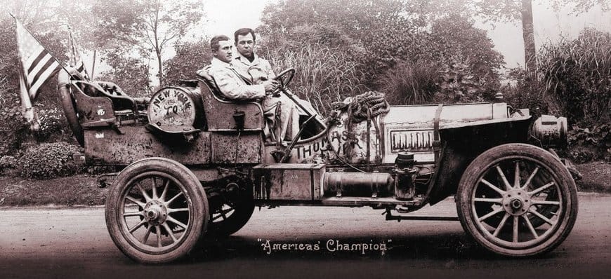
As impressive as Lindberg’s transatlantic fight was in 1926, more impressive was George Schuster driving and winning the New York to Paris Automobile race beginning in the dead of winter, 1908, going the long way, through Russia. As of 1908, only nine cars had ever made the trip from Chicago to California, and none had done it in winter, but this race was to go beyond California, to Alaska and then over the ice through Russia and to Paris. Theodore Roosevelt was president, and Americans were up to any challenge. So, on February 12, 1908 there congregated in Times Square, New York, a single, US-made production car, along with five, specially made super-cars from Europe; one each from Italy and Germany; and three from France. The US car, a Thomas Flyer (white), is shown in the picture below. The ER Thomas company sent along George Schuster, as an afterthought: he was a mechanic and test-driver for the company, and was an ex bicycle racer. The main driver was supposed to be Montague Roberts, a dashing sportsmen, but the fellow dropped out in Cheyenne, Wyoming. Schuster reached the Eiffel tower on July 30, 1908, 169 days after leaving New York. The Germans and Italians followed. None of the French super-cars got further than Vladivostok, and one dropped out after less than 100 miles.

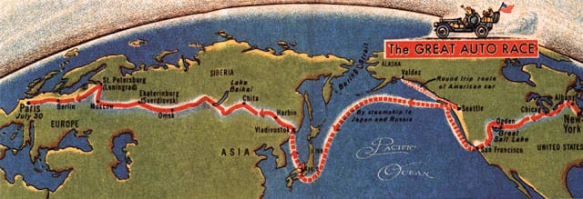
The race was sponsored by The New York Times and Le Matin, a Paris newspaper. They offered a large trophy, a cash prize of $1000, not enough to pay for the race, and the prospect of fame. The original plan was for drivers to go from New York to San Francisco, then to Seattle by ship, and Northern Alaska, driving to Russia across the Arctic ice. That plan was abandoned when Schuster, the first driver to reach Alaska, discovered ten foot snows outside of Valdez. The race was modified so that travel to Russia would be by ship. Schuster took his Thomas to Russia from Alaska, the other two drivers reached Russia from Seattle by way of Japan. Schuster was given a bonus of days to account for having taken the longer route. Because of his detour, he was the last to arrive in Russia. From Japan, the route was Vladivostok, Omsk, Moscow, St. Petersburg, Berlin, and Paris, 21,900 miles total; 13,341 miles driven. Schuster drove most of those 13,341 miles, protected by his own .32-caliber pistol, and mostly guided by the stars and a sextant. He’d taught himself celestial navigation as there were no roadmaps, and hardly any roads.

George Schuster driving the Thomas Flyer, the only American entry, and the only production motorcar in the race.

George Schuster driving the Thomas Flyer with another mechanic, George Miller, the Flyer was only American entry, and the only production motorcar in the race. Note that the flag has only 45 stars.

The ship crossing of the Pacific was a good idea given that, even in the dead of winter, global warming meant that the arctic could not be relied upon to be solid ice. As it was, Schuster had to content with crossing the Rockies in deep snow, and crossing Russia in the season of deepest mud. He reached the Eiffel tower at 6 p.m. on July 30, 1908. The German car had arrived in Paris three days ahead of Schuster, but was penalized to second place because the German team had avoided the trip to Alaska, and had traveled some 150 km of the Western US by railroad while Schuster had driven. The Italian team reached Paris months later, in September, 1908. That the win went to the only production car to compete is indicative, perhaps of the reliability that comes with mass production. That Mr. Schuster was not given the fame that Lindberg got may have to do with the small size of the prize, or with him being a mechanic while Lindberg was a “flyer”. Flyers were sexy; even the car was called a flyer. The Times saw fit to hardly mention Schuster at all, and when it did, it spelled his name wrong. Instead the Times headline read, “Thomas Flyer wins New York to Paris Race.” You’d think the car did it on its own, or that the driver was named Thomas Flyer.

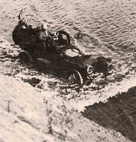
The Flyer crossing a swollen  river in Manchuria.

Schuster in his Flyer crossing a swollen river in Manchuria.

The Times could not get enough of Montague Roberts; the driver of the first leg was famous and photographic. They tried to get Roberts to drive the last few miles into Paris, “once the roads were good”. And Roberts was the one chosen to drive in the hero-parade in New York, Schuster rode too, but didn’t drive. Schuster was feted by Theodore Roosevelt, though, who said he liked people “who did things.” Schuster said he’d never do a race like that again, and he never did race again.

The race did wonders for the reputation of American automobiles, and greatly spurred the desire for roads, but it did little or nothing for the E.R.Thomas company. Thomas cars were high cost, high power models, and they lost out in the marketplace to Henry Ford’s, low-cost Model T’s. You’d think that, in the years leading up to WWI, the US Army might buy a high cost, high reliability car, but they were not interested, and the Thomas company did little to capitalize on their success. The Flyer design that won the race was discontinued. It was a 60 hp, straight 4 cylinder engine version, replaced by lower cost Flyers with 3 cylinders and 24 hp. Shortly after that, Edwin R. Thomas, decided to drop the Flyer altogether. His company went bankrupt in 1912, and was bought by Empire Smelting. The original Flyer was sold in 1913 at a bankruptcy action, lot #1829, “Famous New York to Paris Racer.”

ER Thomas went on to found another car company, as was the style in those days. Thomas-Detroit went on make similar cars to the Flyer, but cheaper. The largest, the K-30, was only 30 hp. The original Thomas Flyer is now in the National Automobile Museum, Reno Nevada. after being identified by Schuster and restored. Here is a video showing the original Flyer being driven by a grandson of George Schuster. There is a lower-power Thomas Flyer (black) in a back space of the Henry Ford museum (Detroit). Protos vehicles, similar to the one that came in second, were produced for the German military through WWI. Their manufacturer, Siemens, benefited, as did the German driver.

Advertisement for the Protos Automobile, a product of Siemens motor company. The race did not include a production Protos but one made specially for the race.

Advertisement for the Protos Automobile, a product of Siemens motor company. The race did not include a production Protos but one made specially for the race.

The Thomas engine (and the Protos) engine) live on in a host of cars with water-cooled, four-cylinder, straight engines. In 1922, Chalmers-Detroit merged with Maxwell and continued to produce versions of the old Flyer design, now with an internal drive-shaft. The original Flyer was powered via a gear-chain, like a bicycle. In 1928, Maxwell was sold to Chrysler. Chrysler persists in calling their high-power, four-cylinder engines by the name Chalmers. As for Schuster, when ER Thomas closed its doors, he had still not been paid for his time as a race driver. He went to work for Pierce-Arrow, another maker of large, heavy vehicles. The “cheaper by the dozen” family (two parents, 12 kids) drove a Pierce-Arrow.

The Great race appears in two documentaries and two general audience movies, both comedies. The first of these was Mishaps of the New York–Paris Race, released by Georges Méliès, July 1908, just about as the Flyer was entering Paris. The second movie version  “The Great Race” was released in 1965. It’s one of my favorite movies, with Jack Lemon as the Protos driver (called Dr. Fate in the movie), Tony Curtis as “The Great Leslie”, the Flyer driver. For the movie, the Flyer is called “The Leslie”, and with Natalie Wood as a female reporter who rides along and provides the love interest. In the actual race reporters from the New York Times, male, traveled in the Flyer’s rear seat sending stories back by carrier pigeon.

Path of the Great Race

Path of the Great Race

As a bit of fame, here’s George Schuster in 1958 on “What’s my secret.” He was 85, and no one knew of him or the race. Ten years later, in 1968, Schuster finally received his $1000 prize, but still no fame. A blow-by-blow of the race can be found here, in Smithsonian magazine. There is also an article about the race in The New York Times, February 10, 2008. This article includes only two pictures, a lead picture showing one of the French cars, and another showing Jeff  Mahl, the grandson of George Schuster, and a tiny bit of the flyer. Why did the New York Times choose these pictures? My guess is it’s the same reason that they reported as they did in 1908: The French car looked better than the Flyer, and Jeff Mahl looked better than George Schuster.

Robert Buxbaum, July 20, 2018. What does all this mean, I’ve wondered as I wrote this essay. There were so many threads, and so many details. After thinking a bit, my take is that the movie versions were right. It was all a comedy. Life becomes a comedy when the wrong person wins, or the wrong vehicle does. A simple mechanic working for a failing auto company beat great drivers and super cars, surpassing all sorts of obstacles that seem impossible to surpass. That’s comedy, It’s for this reason that Dante’s Divine Comedy is a comedy. When we see things like this we half-choose to disbelieve, and we half-choose to laugh, and because we don’t quite believe, very often we don’t reward the winner as happened to Schuster for the 60 years after the race. Roberts should have won, so we’ll half-pretend he did.

Isotopic effects in hydrogen diffusion in metals

For most people, there is a fundamental difference between solids and fluids. Solids have long-term permanence with no apparent diffusion; liquids diffuse and lack permanence. Put a penny on top of a dime, and 20 years later the two coins are as distinct as ever. Put a layer of colored water on top of plain water, and within a few minutes you’ll see that the coloring diffuse into the plain water, or (if you think the other way) you’ll see the plain water diffuse into the colored.

Now consider the transport of hydrogen in metals, the technology behind REB Research’s metallic  membranes and getters. The metals are clearly solid, keeping their shapes and properties for centuries. Still, hydrogen flows into and through the metals at a rate of a light breeze, about 40 cm/minute. Another way of saying this is we transfer 30 to 50 cc/min of hydrogen through each cm2 of membrane at 200 psi and 400°C; divide the volume by the area, and you’ll see that the hydrogen really moves through the metal at a nice clip. It’s like a normal filter, but it’s 100% selective to hydrogen. No other gas goes through.

To explain why hydrogen passes through the solid metal membrane this way, we have to start talking about quantum behavior. It was the quantum behavior of hydrogen that first interested me in hydrogen, some 42 years ago. I used it to explain why water was wet. Below, you will find something a bit more mathematical, a quantum explanation of hydrogen motion in metals. At REB we recently put these ideas towards building a membrane system for concentration of heavy hydrogen isotopes. If you like what follows, you might want to look up my thesis. This is from my 3rd appendix.

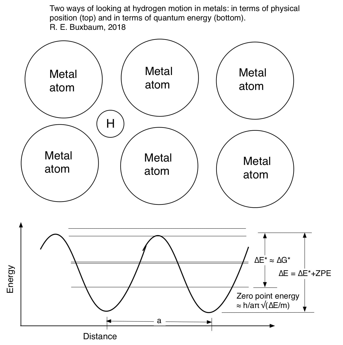
Although no-one quite understands why nature should work this way, it seems that nature works by quantum mechanics (and entropy). The basic idea of quantum mechanics you will know that confined atoms can only occupy specific, quantized energy levels as shown below. The energy difference between the lowest energy state and the next level is typically high. Thus, most of the hydrogen atoms in an atom will occupy only the lower state, the so-called zero-point-energy state.

A hydrogen atom, shown occupying an interstitial position between metal atoms (above), is also occupying quantum states (below). The lowest state, ZPE is above the bottom of the well. Higher energy states are degenerate: they appear in pairs. The rate of diffusive motion is related to ∆E* and this degeneracy.

A hydrogen atom, shown occupying an interstitial position between metal atoms (above), is also occupying quantum states (below). The lowest state, ZPE is above the bottom of the well. Higher energy states are degenerate: they appear in pairs. The rate of diffusive motion is related to ∆E* and this degeneracy.

The fraction occupying a higher energy state is calculated as c*/c = exp (-∆E*/RT). where ∆E* is the molar energy difference between the higher energy state and the ground state, R is the gas constant and T is temperature. When thinking about diffusion it is worthwhile to note that this energy is likely temperature dependent. Thus ∆E* = ∆G* = ∆H* – T∆S* where asterisk indicates the key energy level where diffusion takes place — the activated state. If ∆E* is mostly elastic strain energy, we can assume that ∆S* is related to the temperature dependence of the elastic strain.

Thus,

∆S* = -∆E*/Y dY/dT

where Y is the Young’s modulus of elasticity of the metal. For hydrogen diffusion in metals, I find that ∆S* is typically small, while it is often typically significant for the diffusion of other atoms: carbon, nitrogen, oxygen, sulfur…

The rate of diffusion is now calculated assuming a three-dimensional drunkards walk where the step lengths are constant = a. Rayleigh showed that, for a simple cubic lattice, this becomes:

D = a2/6τ

a is the distance between interstitial sites and t is the average time for crossing. For hydrogen in a BCC metal like niobium or iron, D=

a2/9τ; for a FCC metal, like palladium or copper, it’s

a2/3τ. A nice way to think about τ, is to note that it is only at high-energy can a hydrogen atom cross from one interstitial site to another, and as we noted most hydrogen atoms will be at lower energies. Thus,

τ = ω c*/c = ω exp (-∆E*/RT)

where ω is the approach frequency, or the amount of time it takes to go from the left interstitial position to the right one. When I was doing my PhD (and still likely today) the standard approach of physics writers was to use a classical formulation for this time-scale based on the average speed of the interstitial. Thus, ω = 1/2a√(kT/m), and

τ = 1/2a√(kT/m) exp (-∆E*/RT).

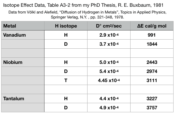
In the above, m is the mass of the hydrogen atom, 1.66 x 10⁻²⁴ g for protium, and twice that for deuterium, etc., a is the distance between interstitial sites, measured in cm, T is temperature, Kelvin, and k is the Boltzmann constant, 1.38 x 10⁻¹⁶ erg/°K. This formulation correctly predicts that heavier isotopes will diffuse slower than light isotopes, but it predicts incorrectly that, at all temperatures, the diffusivity of deuterium is 1/√2 that for protium, and that the diffusivity of tritium is 1/√3 that of protium. It also suggests that the activation energy of diffusion will not depend on isotope mass. I noticed that neither of these predictions is borne out by experiment, and came to wonder if it would not be more correct to assume ω represent the motion of the lattice, breathing, and not the motion of a highly activated hydrogen atom breaking through an immobile lattice. This thought is borne out by experimental diffusion data where you describe hydrogen diffusion as D = D° exp (-∆E*/RT).

Screen Shot 2018-06-21 at 12.08.20 AM

You’ll notice from the above that D° hardly changes with isotope mass, in complete contradiction to the above classical model. Also note that ∆E* is very isotope dependent. This too is in contradiction to the classical formulation above. Further, to the extent that D° does change with isotope mass, D° gets larger for heavier mass hydrogen isotopes. I assume that small difference is the entropy effect of ∆E* mentioned above. There is no simple square-root of mass behavior in contrast to most of the books we had in grad school.

As for why ∆E* varies with isotope mass, I found that I could get a decent explanation of my observations if I assumed that the isotope dependence arose from the zero point energy. Heavier isotopes of hydrogen will have lower zero-point energies, and thus ∆E* will be higher for heavier isotopes of hydrogen. This seems like a far better approach than the semi-classical one, where ∆E* is isotope independent.

I will now go a bit further than I did in my PhD thesis. I’ll make the general assumption that the energy well is sinusoidal, or rather that it consists of two parabolas one opposite the other. The ZPE is easily calculated for parabolic energy surfaces (harmonic oscillators). I find that ZPE = h/aπ √(∆E/m) where m is the mass of the particular hydrogen atom, h is Plank’s constant, 6.63 x 10⁻²⁷ erg-sec,  and ∆E is ∆E* + ZPE, the zero point energy. For my PhD thesis, I didn’t think to calculate ZPE and thus the isotope effect on the activation energy. I now see how I could have done it relatively easily e.g. by trial and error, and a quick estimate shows it would have worked nicely. Instead, for my PhD, Appendix 3, I only looked at D°, and found that the values of D° were consistent with the idea that ω is about 0.55 times the Debye frequency, ω ≈ .55 ωD. The slight tendency for D° to be larger for heavier isotopes was explained by the temperature dependence of the metal’s elasticity.

Two more comments based on the diagram I presented above. First, notice that there is middle split level of energies. This was an explanation I’d put forward for quantum tunneling atomic migration that some people had seen at energies below the activation energy. I don’t know if this observation was a reality or an optical illusion, but present I the energy picture so that you’ll have the beginnings of a description. The other thing I’d like to address is the question you may have had — why is there no zero-energy effect at the activated energy state. Such a zero energy difference would cancel the one at the ground state and leave you with no isotope effect on activation energy. The simple answer is that all the data showing the isotope effect on activation energy, table A3-2, was for BCC metals. BCC metals have an activation energy barrier, but it is not caused by physical squeezing between atoms, as for a FCC metal, but by a lack of electrons. In a BCC metal there is no physical squeezing, at the activated state so you’d expect to have no ZPE there. This is not be the case for FCC metals, like palladium, copper, or most stainless steels. For these metals there is a much smaller, on non-existent isotope effect on ∆E*.

Robert Buxbaum, June 21, 2018. I should probably try to answer the original question about solids and fluids, too: why solids appear solid, and fluids not. My answer has to do with quantum mechanics: Energies are quantized, and always have a ∆E* for motion. Solid materials are those where ω exp (-∆E*/RT) has unit of centuries. Thus, our ability to understand the world is based on the least understandable bit of physics.

Alkaline batteries have second lives

Most people assume that alkaline batteries are one-time only, throwaway items. Some have used rechargeable cells, but these are Ni-metal hydride, or Ni-Cads, expensive variants that have lower power densities than normal alkaline batteries, and almost impossible to find in stores. It would be nice to be able to recharge ordinary alkaline batteries, e.g. when a smoke alarm goes off in the middle of the night and you find you’re out, but people assume this is impossible. People assume incorrectly.

Modern alkaline batteries are highly efficient: more efficient than even a few years ago, and that always suggests reversibility. Unlike the acid batteries you learned about in highschool chemistry class (basic chemistry due to Volta) the chemistry of modern alkaline batteries is based on Edison’s alkaline car batteries. They have been tweaked to an extent that even the non-rechargeable versions can be recharged. I’ve found I can reliably recharge an ordinary alkaline cell, 9V, at least once using the crude means of a standard 12 V car battery charger by watching the amperage closely. It only took 10 minutes. I suspect I can get nine lives out of these batteries, but have not tried.

To do this experiment, I took a 9 V alkaline that had recently died, and finding I had no replacement, I attached it to a 6 Amp, 12 V, car battery charger that I had on hand. I would have preferred to use a 2 A charger and ideally a charger designed to output 9-10 V, but a 12 V charger is what I had available, and it worked. I only let it charge for 10 minutes because, at that amperage, I calculated that I’d recharged to the full 1 Amp-hr capacity. Since the new alkaline batteries only claimed 1 amp hr, I figured that more charge would likely do bad things, even perhaps cause the thing to blow up.  After 5 minutes, I found that the voltage had returned to normal and the battery worked fine with no bad effects, but went for the full 10 minutes. Perhaps stopping at 5 would have been safer.

I changed for 10 minutes (1/6 hour) because the battery claimed a capacity of 1 Amp-hour when new. My thought was 1 amp-hour = 1 Amp for 1 hour, = 6 Amps for 1/6 hour = ten minutes. That’s engineering math for you, the reason engineers earn so much. I figured that watching the recharge for ten minutes was less work and quicker than running to the store (20 minutes). I used this battery in my firm alarm, and have tested it twice since then to see that it works. After a few days in my fire alarm, I took it out and checked that the voltage was still 9 V, just like when the battery was new. Confirming experiments like this are a good idea. Another confirmation occurred when I overcooked some eggs and the alarm went off from the smoke.

If you want to experiment, you can try a 9V as I did, or try putting a 1.5 volt AA or AAA battery in a charger designed for rechargeables. Another thought is to see what happens when you overcharge. Keep safe: do this in a wood box outside at a distance, but I’d like to know how close I got to having an exploding energizer. Also, it would be worthwhile to try several charge/ discharge cycles to see how the energy content degrades. I expect you can get ~9 recharges with a “non-rechargeable” alkaline battery because the label says: “9 lives,” but even getting a second life from each battery is a significant savings. Try using a charger that’s made for rechargeables. One last experiment: If you’ve got a cell phone charger that works on a car battery, and you get the polarity right, you’ll find you can use a 9V alkaline to recharge your iPhone or Android. How do I know? I judged a science fair not long ago, and a 4th grader did this for her science fair project.

Robert Buxbaum, April 19, 2018. For more, semi-dangerous electrochemistry and biology experiments.

What drives the gulf stream?

I’m not much of a fan of todays’ kids’ science books because they don’t teach science IMHO. They have nice pictures and a few numbers; almost no equations, and lots of words. You can’t do science that way. On the odd occasion that they give the right answer to some problem, the lack of math means the kid has no way of understanding the reasoning, and no reason to believe the answer. Professional science articles on the web are bad in the opposite direction: too many numbers and for math, hey rely on supercomputers. No human can understand the outcome. I like to use my blog to offer science with insight, the type you’d get in an old “everyman science” book.

In previous posts, I gave answers to why the sky is blue, why it’s cold at the poles, why it’s cold on mountains, how tornadoes pick stuff up, and why hurricanes blow the way they do. In this post, we’ll try to figure out what drives the gulf-stream. The main argument will be deduction — disproving things that are not driving the gulf stream to leave us with one or two that could. Deduction is a classic method of science, well presented by Sherlock Holmes.

The gulf stream. The speed in the white area is ≥ 0.5 m/s (1.1 mph.).

The gulf stream. The speed in the white area is ≥ 0.5 m/s (1.1 mph.).

For those who don’t know, the Gulf stream is a massive river of water that runs within the Atlantic ocean. As shown at right, it starts roughly at the end of Florida, runs north to the Carolinas, and then turns dramatically east towards Spain. Flowing east, It’s about 150 miles wide, but only about 62 miles (100 km) when flowing along the US coast. According to some of the science books of my youth this massive flow was driven by temperature according to others, by salinity (whatever that means), and yet other books of my youth wind. My conclusion: they had no clue.

As a start to doing the science here, it’s important to fill in the numerical information that the science books left out. The Gulf stream is roughly 1000 meters deep, with a typical speed of 1 m/s (2.3 mph). The maximum speed is the surface water as the stream flows along the US coast. It is about 2.5 metres per second (5.6 mph), see map above.

From the size and the speed of the Gulf Stream, we conclude that land rivers are not driving the flow. The Mississippi is a big river with an outflow point near the head waters of the gulf stream, but the volume of flow is vastly too small. The volume of the gulf stream is roughly

Q=wdv = 100,000 x 1000 x .5 =  50 million m3/s = 1.5 billion cubic feet/s.

This is about 2000 times more flow than the volume flow of the Mississippi, 18,000 m3/s. The great difference in flow suggests the Mississippi could not be the driving force. The map of flow speeds (above) also suggest rivers do not drive the flow. The Gulf Stream does not flow at its maximum speed near the mouth of any river.  We now look for another driver.

Moving on to temperature. Temperature drives the whirl of hurricanes. The logic for temperature driving the gulf stream is as follows: it’s warm by the equator and cold at the poles; warm things expand and as water flows downhill, the polls will always be downhill from the equator. Lets put some math in here or my explanation will be lacking. First lets consider how much hight difference we might expect to see. The thermal expansivity of water is about 2x 10⁻⁴ m/m°C (.0002/°C) in the desired temperature range). To calculate the amount of expansion we multiply this by the depth of the stream, 1000m, and the temperature difference between two points, eg. the end of Florida to the Carolina coast. This is 5°C (9°F) I estimate. I calculate the temperature-induced seawater height as:

∆h (thermal) ≈ 5° x .0002/° x 1000m = 1 m (3.3 feet).

This is a fair amount of height. It’s only about 1/100 the height driving the Mississippi river, but it’s something. To see if 1 m is enough to drive the Gulf flow, I’ll compare it to the velocity-head. Velocity-head is a concept that’s useful in plumbing (I ran for water commissioner). It’s the potential energy height equivalent of any kinetic energy — typically of a fluid flow. The kinetic energy for any velocity v and mass of water, m is 1/2 mv2 . The potential energy equivalent is mgh. Combine the above and remove the mass terms, and we have:

∆h (velocity) = v2/2g.

Where g is the acceleration of gravity. Let’s consider  v = 1 m/s and g= 9.8 m/s2.≤ 0.05 m ≈ 2 inches. This is far less than the driving force calculated above. We have 5x more driving force than we need, but there is a problem: why isn’t the flow faster? Why does the Mississippi move so slowly when it has 100 times more head.

To answer the above questions, and to check if heat could really drive the Gulf Stream, we’ll check if the flow is turbulent — it is. A measure of how turbulent is based on something called the Reynolds number, Re#, it’s the ratio of kinetic energy and viscous loss in a fluid flow. Flows are turbulent if this ratio is more than 3000, or so;

Re# = vdρ/µ.

In the above, v is velocity, say 1 m/s, d is depth, 1000m, ρ = density, 1000 kg/m3 for water, and  0.00133 Pa∙s is the viscosity of water. Plug in these numbers, and we find a RE# = 750 million: this flow will be highly turbulent. Assuming a friction factor of 1/20 (.05), e find that we’d expect complete mixing 20 depths or 20 km. We find we need the above 0.05 m of velocity height to drive every 20 km of flow up the US coast. If the distance to the Carolina coast is 1000 km we need 1000*.05m/20 = 1 meter, that’s just about the velocity-head that the temperature difference would suggest. Temperature is thus a plausible driving force for 0.5 m/s, though not likely for the faster 2.5 m/s flow seen in the center of the stream. Turbulent flow is a big part of figuring the mpg of an automobile; it becomes rapidly more important at high speeds.

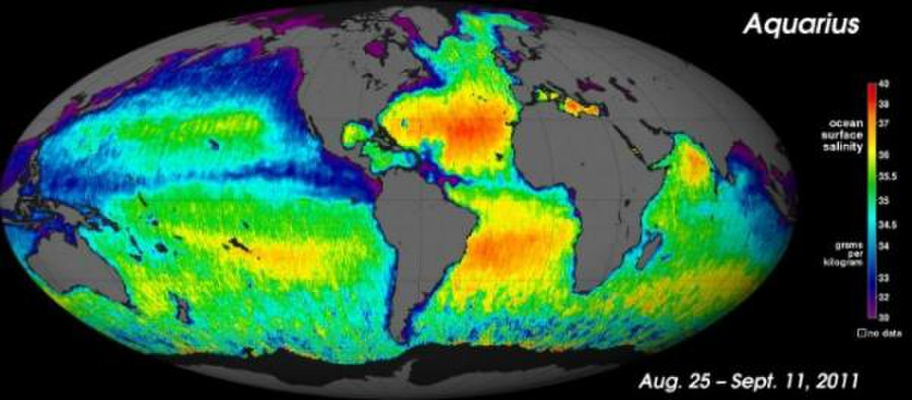
World sea salinity

World sea salinity. The maximum and minimum are in the wrong places.

What about salinity? For salinity to work, the salinity would have to be higher at the end of the flow. As a model of the flow, we might imagine that we freeze arctic seawater, and thus we concentrate salt in the seawater just below the ice. The heavy, saline water would flow down to the bottom of the sea, and then flow south to an area of low salinity and low pressure. Somewhere in the south, the salinity would be reduced by rains. If evaporation were to exceed the rains, the flow would go in the other direction. Sorry to say, I see no evidence of any of this. For one the end of the Gulf Stream is not that far north; there is no freezing, For two other problems: there are major rains in the Caribbean, and rains too in the North Atlantic. Finally, while the salinity head is too small. Each pen of salinity adds about 0.0001g/cc, and the salinity difference in this case is less than 1 ppm, lets say 0.5ppm.

h = .0001 x 0.5 x 1000 = 0.05m

I don’t see a case for northern-driven Gulf-stream flow caused by salinity.

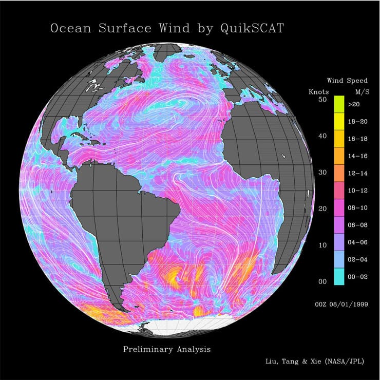
Surface level winds in the Atlantic.

Surface level winds in the Atlantic. Trade winds in purple, 15-20 mph.

Now consider winds. The wind velocities are certainly enough to produce 5+ miles per hour flows, and the path of flows is appropriate. Consider, for example, the trade winds. In the southern Caribbean, they blow steadily from east to west slightly above the equator at 15 -20 mph. This could certainly drive a circulation flow of 4.5 mph north. Out of the Caribbean basin and along the eastern US coat the trade winds blow at 15-50 mph north and east. This too would easily drive a 4.5 mph flow.  I conclude that a combination of winds and temperature are the most likely drivers of the gulf stream flow. To quote Holmes, once you’ve eliminated the impossible, whatever remains, however improbable, must be the truth.

Robert E. Buxbaum, March 25, 2018. I used the thermal argument above to figure out how cold it had to be to freeze the balls off of a brass monkey.

Keeping your car batteries alive.

Lithium-battery cost and performance has improved so much that no one uses Ni-Cad or metal hydride batteries any more. These are the choice for tools, phones, and computers, while lead acid batteries are used for car starting and emergency lights. I thought I’d write about the care and trade-offs of these two remaining options.

As things currently stand, you can buy a 12 V, lead-acid car battery with 40 Amp-h capacity for about $95. This suggests a cost of about $200/ kWh. The price rises to $400/kWh if you only discharge half way (good practice). This is cheaper than the per-power cost of lithium batteries, about $500/ kWh or $1000/ kWh if you only discharge half-way (good practice), but people pick lithium because (1) it’s lighter, and (2) it’s generally longer lasting. Lithium generally lasts about 2000 half-discharge cycles vs 500 for lead-acid.

On the basis of cost per cycle, lead acid batteries would have been replaced completely except that they are more tolerant of cold and heat, and they easily output the 400-800 Amps needed to start a car. Lithium batteries have problems at these currents, especially when it’s hot or cold. Lithium batteries deteriorate fast in the heat too (over 40°C, 105°F), and you can not charge a lithium car battery at more than 3-4 Amps at temperatures below about 0°C, 32°F. At higher currents, a coat of lithium metal forms on the anode. This lithium can react with water: 2Li + H2O –> Li2O + H2, or it can form dendrites that puncture the cell separators leading to fire and explosion. If you charge a lead acid battery too fast some hydrogen can form, but that’s much less of a problem. If you are worried about hydrogen, we sell hydrogen getters and catalysts that remove it. Here’s a description of the mechanisms.

The best thing you can do to keep a lead-acid battery alive is to keep it near-fully charged. This can be done by taking long drives, by idling the car (warming it up), or by use of an external trickle charger. I recommend a trickle charger in the winter because it’s non-polluting. A lead-acid battery that’s kept at near full charge will give you enough charge for 3000 to 5000 starts. If you let the battery completely discharge, you get only 50 or so deep cycles or 1000 starts. But beware: full discharge can creep up on you. A new car battery will hold 40 Ampere-hours of current, or 65,000 Ampere-seconds if you half discharge. Starting the car will take 5 seconds of 600 Amps, using 3000 Amp-s or about 5% of the battery’s juice. The battery will recharge as you drive, but not that fast. You’ll have to drive for at least 500 seconds (8 minutes) to recharge from the energy used in starting. But in the winter it is common that your drive will be shorter, and that a lot of your alternator power will be sent to the defrosters, lights, and seat heaters. As a result, your lead-acid battery will not totally charge, even on a 10 minute drive. With every week of short trips, the battery will drain a little, and sooner or later, you’ll find your battery is dead. Beware and recharge, ideally before 50% discharge

A little chemistry will help explain why full discharging is bad for battery life (for a different version see Wikipedia). For the first half discharge of a lead-acid battery, the reaction Is:

Pb + 2PbO2 + 2H2SO4  –> PbSO4 + Pb2O2SO4 + 2H2O.

This reaction involves 2 electrons and has a -∆G° of >394 kJ, suggesting a reversible voltage more than 2.04 V per cell with voltage decreasing as H2SO4 is used up. Any discharge forms PbSO4 on the positive plate (the lead anode) and converts lead oxide on the cathode (the negative plate) to Pb2O2SO4. Discharging to more than 50% involves this reaction converting the Pb2O2SO4 on the cathode to PbSO4.

Pb + Pb2O2SO4 + 2H2SO4  –> 2PbSO4 + 2H2O.

This also involves two electrons, but -∆G < 394 kJ, and voltage is less than 2.04 V. Not only is the voltage less, the maximum current is less. As it happens Pb2O2SO4 is amorphous, adherent, and conductive, while PbSO4 is crystalline, not that adherent, and not-so conductive. Operating at more than 50% results in less voltage, increased internal resistance, decreased H2SO4 concentrations, and lead sulfate flaking off the electrode. Even letting a battery sit at low voltage contributes to PbSO4 flaking off. If the weather is cold enough, the low concentration H2SO4 freezes and the battery case cracks. My advice: Get out your battery charger and top up your battery. Don’t worry about overcharging; your battery charger will sense when the charge is complete. A lead-acid battery operated at near full charge, between 67 and 100% will provide 1500 cycles, about as many as lithium. 

Trickle charging my wife's car. Good for battery life. At 6 Amps, expect this to take 3-6 hours.

Trickle charging my wife’s car: good for battery life. At 6 Amps, expect a full charge to take 6 hours or more. You might want to recharge the battery in your emergency lights too. 

Lithium batteries are the choice for tools and electric vehicles, but the chemistry is different. For longest life with lithium batteries, they should not be charged fully. If you change fully they deteriorate and self-discharge, especially when warm (100°F, 40°C). If you operate at 20°C between 75% and 25% charge, a lithium-ion battery will last 2000 cycles; at 100% to 0%, expect only 200 cycles or so.

Tesla cars use lithium batteries of a special type, lithium cobalt. Such batteries have been known to explode, but and Tesla adds sophisticated electronics and cooling systems to prevent this. The Chevy Volt and Bolt use lithium batteries too, but they are less energy-dense. In either case, assuming $1000/kWh and a 2000 cycle life, the battery cost of an EV is about 50¢/kWh-cycle. Add to this the cost of electricity, 15¢/kWh including the over-potential needed to charge, and I find a total cost of operation of 65¢/kWh. EVs get about 3 miles per kWh, suggesting an energy cost of about 22¢/mile. By comparison, a 23 mpg car that uses gasoline at $2.80 / gal, the energy cost is 12¢/mile, about half that of the EVs. For now, I stick to gasoline for normal driving, and for long trips, suggest buses, trains, and flying.

Robert Buxbaum, January 4, 2018.

Hydrogen permeation rates in Inconel, Hastelloy and stainless steels.

Some 20 years ago, I published a graph of the permeation rate for hydrogen in several metals at low pressure, See the graph here, but I didn’t include stainless steel in the graph.

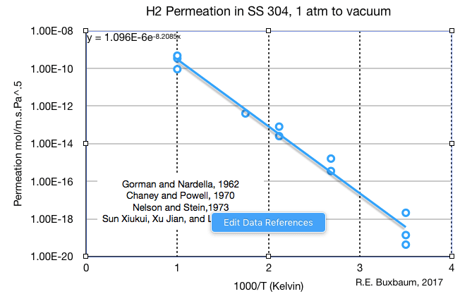
Hydrogen permeation in clean SS-304; four research groups’ data.

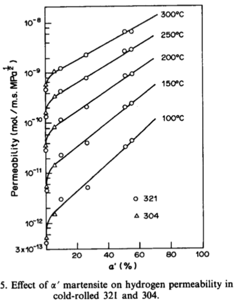
One reason I did not include stainless steel was there were many stainless steels and the hydrogen permeation rates were different, especially so between austenitic (FCC) steels and ferritic steels (BCC). Another issue was oxidation. All stainless steels are oxidized, and it affect H2 permeation a lot. You can decrease the hydrogen permeation rate significantly by oxidation, or by surface nitriding, etc (my company will even provide this service). Yet another issue is cold work. When  an austenitic stainless steel is worked — rolled or drawn — some Austinite (FCC) material transforms to Martisite (a sort of stretched BCC). Even a small amount of martisite causes an order of magnitude difference in the permeation rate, as shown below. For better or worse, after 20 years, I’m now ready to address H2 in stainless steel, or as ready as I’m likely to be.

Hydrogen permeation data for SS 340 and SS 321.

Hydrogen permeation in SS 340 and SS 321. Cold work affects H2 permeation more than the difference between 304 and 321; Sun Xiukui, Xu Jian, and Li Yiyi, 1989

The first graph I’d like to present, above, is a combination of four research groups’ data for hydrogen transport in clean SS 304, the most common stainless steel in use today. SS 304 is a ductile, austenitic (FCC), work hardening, steel of classic 18-8 composition (18% Cr, 8% Ni). It shares the same basic composition with SS 316, SS 321 and 304L only differing in minor components. The data from four research groups shows a lot of scatter: a factor of 5 variation at high temperature, 1000 K (727 °C), and almost two orders of magnitude variation (factor of 50) at room temperature, 13°C. Pressure is not a factor in creating the scatter, as all of these studies were done with 1 atm, 100 kPa hydrogen transporting to vacuum.

The two likely reasons for the variation are differences in the oxide coat, and differences in the amount of cold work. It is possible these are the same explanation, as a martensitic phase might increase H2 permeation by introducing flaws into the oxide coat. As the graph at left shows, working these alloys causes more differences in H2 permeation than any difference between alloys, or at least between SS 304 and SS 321. A good equation for the permeation behavior of SS 304 is:

P (mol/m.s.Pa1/2) = 1.1 x10⁻⁶ exp (-8200/T).      (H2 in SS-304)

Because of the song influence of cold work and oxidation, I’m of the opinion that I get a slightly different, and better equation if I add in permeation data from three other 18-8 stainless steels:

P (mol/m.s.Pa1/2) = 4.75 x10-7 exp (-7880/T).     (H2 in annealed SS-304, SS-316, SS-321)

Screen Shot 2017-12-16 at 10.37.37 PM

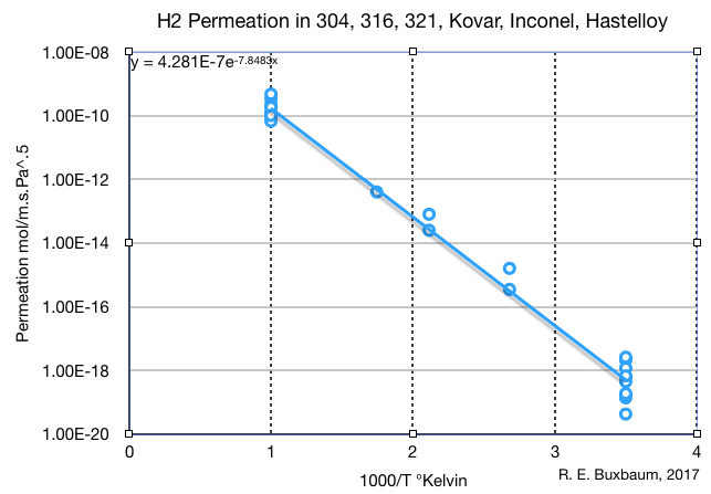
Hydrogen permeation through several common stainless steels, as well as Inocnel and Hastelloy

Though this result is about half of the previous at high temperature, I would trust it better, at least for annealed SS-304, and also for any annealed austenitic stainless steel. Just as an experiment, I decided to add a few nickel and cobalt alloys to the mix, and chose to add data for inconel 600, 625, and 718; for kovar; for Hastelloy, and for Fe-5%Si-5%Ge, and SS4130. At left, I pilot all of these on one graph along with data for the common stainless steels. To my eyes the scatter in the H2 permeation rates is indistinguishable from that SS 304 above or in the mixed 18-8 steels (data not shown). Including these materials to the plot decreases the standard deviation a bit to a factor of 2 at 1000°K and a factor of 4 at 13°C. Making a least-square analysis of the data, I find the following equation for permeation in all common FCC stainless steels, plus Inconels, Hastelloys and Kovar:

P (mol/m.s.Pa1/2) = 4.3 x10⁻⁷ exp (-7850/T).

This equation is near-identical to the equation above for mixed, 18-8 stainless steel. I would trust it for annealed or low carbon metal (SS-304L) to a factor of 2 accuracy at high temperatures, or a factor of 4 at low temperatures. Low carbon reduces the tendency to form Martinsite. You can not use any of these equations for hydrogen in ferritic (BCC) alloys as the rates are different, but this is as good as you’re likely to get for basic austenitc stainless and related materials. If you are interested in the effect of cold work, here is a good reference. If you are bothered by the square-root of pressure driving force, it’s a result of entropy: hydrogen travels in stainless steel as dislocated H atoms and the dissociation H2 –> 2 H leads to the square root.

Robert Buxbaum, December 17, 2017. My business, REB Research, makes hydrogen generators and purifiers; we sell getters; we consult on hydrogen-related issues, and will (if you like) provide oxide (and similar) permeation barriers.

Change home air filters 3 times per year

Energy efficient furnaces use a surprisingly large amount of electricity to blow the air around your house. Part of the problem is the pressure drop of the ducts, but quite a lot of energy is lost bowing air through the dust filter. An energy-saving idea: replace the filter on your furnace twice a year or more. Another idea, you don’t have to use the fanciest of filters. Dirty filters provide a lot of back-pressure especially when they are dirty.

I built a water manometer, see diagram below to measure the pressure drop through my furnace filters. The pressure drop is measured from the difference in the height of the water column shown. Each inch of water is 0.04 psi or 275 Pa. Using this pressure difference and the flow rating of the furnace, I calculated the amount of power lost by the following formula:

W = Q ∆P/ µ.

Here W is the amount of power use, Watts, Q is flow rate m3/s, ∆P = the pressure drop in Pa, and µ is the efficiency of the motor and blower, typically about 50%.

With clean filters (two different brands), I measured 1/8″ and 1/4″ of water column, or a pressure drop of 0.005 and 0.01 psi, depending on the filter. The “better the filter”, that is the higher the MERV rating, the higher the pressure drop. I also measured the pressure drop through a 6 month old filter and found it to be 1/2″ of water, or 0.02 psi or 140 Pa. Multiplying this by the amount of air moved, 1000 cfm =  25 m3 per minute or 0.42 m3/s, and dividing by the efficiency, I calculate a power use of 118 W. That is 0.118 kWh/hr. or 2.8 kWh/day.

water manometer used to measure pressure drop through the filter of my furnace. I stuck two copper tubes into the furnace, and attached a plastic hose. Pressure was measured from the difference in the water level in the hose.

The water manometer I used to measure the pressure drop through the filter of my furnace. I stuck two copper tubes into the furnace, and attached a plastic tube half filled with water between the copper tubes. Pressure was measured from the difference in the water level in the plastic tube. Each 1″ of water is 280 Pa or 0.04psi.

At the above rate of power use and a cost of electricity of 11¢/kWhr, I find it would cost me an extra 4 KWhr or about 31¢/day to pump air through my dirty-ish filter; that’s $113/year. The cost through a clean filter would be about half this, suggesting that for every year of filter use I spend an average of $57t where t is the use life of the filter.

To calculate the ideal time to change filters I set up the following formula for the total cost per year $, including cost per year spent on filters (at $5/ filter), and the pressure-induced electric cost:

$ = 5/t + 57 t.

The shorter the life of the filter, t, the more I spend on filters, but the less on electricity. I now use calculus to find the filter life that produces the minimum $, and determine that $ is a minimum at a filter life t = √5/57 = .30 years.  The upshot, then, if you filters are like mine, you should change your three times a year, or so; every 3.6 months to be super-exact. For what it’s worth, I buy MERV 5 filters at Ace or Home Depot. If I bought more expensive filters, the optimal change time would likely be once or twice per year. I figure that, unless you are very allergic or make electronics in your basement you don’t need a filter with MERV rating higher than 8 or so.

I’ve mentioned in a previous essay/post that dust starts out mostly as dead skin cells. Over time dust mites eat the skin, some pretty nasty stuff. Most folks are allergic to the mites, but I’m not convinced that the filter on your furnace dies much to isolate you from them since the mites, etc tend to hang out in your bed and clothes (a charming thought, I know).

Old fashioned, octopus furnace. Free convection.

Old fashioned, octopus furnace. Free convection.

The previous house I had, had no filter on the furnace (and no blower). I noticed no difference in my tendency to cough or itch. That furnace relied for circulation on the tendency for hot air to rise. That is, “free convection” circulated air through the home and furnace by way of “Octopus” ducts. If you wonder what a furnace like that looks like here’s a picture.

I calculate that a 10 foot column of air that is 30°C warmer than that in a house will have a buoyancy of about 0.00055 psi (1/8″ of water). That’s enough pressure to drive circulation through my home, and might have even driven air through a clean, low MERV dust filter. The furnace didn’t use any more gas than a modern furnace would, as best I could tell, since I was able to adjust the damper easily (I could see the flame). It used no electricity except for the thermostat control, and the overall cost was lower than for my current, high-efficiency furnace with its electrical blower and forced convection.

Robert E. Buxbaum, December 7, 2017. I ran for water commissioner, and post occasional energy-saving or water saving ideas. Another good energy saver is curtains. And here are some ideas on water-saving, and on toilet paper.

Forced diversity of race is racist

Let me browse through some thoughts on efforts to address endemic racism. I’m not sure I’ll get anywhere, but you might as well enter the laboratory of my mind on the issue.

I’d like to begin with a line of the bible (why not?) “‘Do not pervert justice; do not show partiality to the poor or favoritism to the great, but judge your neighbor fairly.” (Lev. 19:15). This sounds good, but in college admissions, I’ve found we try to do better by showing  favoritism to the descendants of those who’ve been historically left-out. This was called affirmative action, it’s now called “diversity”.  

In 1981, when I began teaching chemical engineering at Michigan State University, our department had race-based quotas to allow easier admission to the descendants of historically-disadvantaged groups. All major universities did this at the time. The claim was that it would be temporary; it continues to this day. In our case, the target was to get 15% or so black, Hispanics and American Indians students (7 in a class of 50). We achieved this target by accepting such students with a 2.0 GPA, and not requiring a math or science background; Caucasians required 3.0 minimum, and we did require math or science. I’m not sure we helped the disadvantaged by this, either personally or professionally, but we made the administration happy. The kids seemed happy too, at least for a while. The ones we got were, by and large, bright. To make up for the lack of background we offered tutoring and adjusted grades. Some diversity students did well, others didn’t. Mostly they went into HR or management after graduation, places they could have gone without our efforts.

After some years, the Supreme court ended our quota based selection, saying it was, itself racist. They said we could still reverse-discriminate for “diversity,” though. That is, if the purpose wasn’t to address previous wrongs, but to improve the class. We changed our literature, but kept our selection methods and kept the same percentage targets as before.

This is a popular meme about racism. It makes sense to me.

This is a popular meme about racism.

The only way we monitored that we met the race-percent target was by a check-box on forms. Students reported race, and we collected this, but we didn’t check that black students look black or Hispanic students spoke Spanish. There was no check on student honesty. Anyone who checked the box got the benefits. This lack of check bread cheating at MSU and elsewhere. Senator Elizabeth Warren got easy entry into Harvard and Penn, in part by claiming to be an Indian on her forms. She has no evidence of Indian blood or culture Here’s Snopes. My sense is that our methods mostly help the crooked.

The main problem with is, I suspect, is the goal. We’ve decided to make every university department match the state’s racial breakdown. It’s a pretty goal, but it doesn’t seem like one that helps students or the state. Would it help the MSU hockey squad to force to team to racially match the state; would it help the volleyball team, or the football team?  So why assume it helps every academic department to make it’s racial makeup match the state’s. Why not let talented black students head to business or management departments before graduation. They might go further without our intervention.

This is not to say there are not racial inequalities, but I suspect that these diversity programs don’t help the students, and may actually hurt. They promote crookedness, and divert student attention from achieving excellence to maintaining victim status. Any group that isn’t loud enough in claiming victim status is robbed of the reverse-discrimination that they’ve been told they need. They’re told they can’t really compete, and many come to believe it. In several universities, we gone so far as to hire “bias referees” to protect minorities from having to defend their intellectual views in open discussion. The referee robs people of the need to think, and serves, I suspect, no one but a group of powerful politicians and administrators — people you are not supposed to criticize. On that topic, here is a video of Malcolm X talking about the danger of white liberals. Clearly he can hold his own in a debate without having a bias referee, and he makes some very good points about white liberals doing more harm than good.

Robert Buxbaum, November 5, 2017. In a related problem, black folks are arrested too often. I suggest rational drug laws. Some financial training could help too.

How Tesla invented, I think, Tesla coils and wireless chargers.

I think I know how Tesla invented his high frequency devices, and thought I’d show you, while also explaining the operation of some devices that develop from in. Even if I’m wrong in historical terms, at least you should come to understand some of his devices, and something of the invention process. Either can be the start of a great science fair project.

physics drawing of a mass on a spring, left, and of a grounded capacitor and inception coil, right.

The start of Tesla’s invention process, I think, was a visual similarity– I’m guessing he noticed that the physics symbol for a spring was the same as for an electrical, induction coil, as shown at left. A normal person would notice the similarity, and perhaps think about it for a few seconds, get no where, and think of something else. If he or she had a math background — necessary to do most any science — they might look at the relevant equations and notice that they’re different. The equation describing the force of a spring is F = -k x  (I’ll define these letters in the bottom paragraph). The equation describing the voltage in an induction coil is not very similar-looking at first glance, V = L di/dt.  But there is a key similarity that could appeal to some math aficionados: both equations are linear. A linear equation is one where, if you double one side you double the other. Thus, if you double F, you double x, and if you double V, you double dI/dt, and that’s a significant behavior; the equation z= atis not linear, see the difference?

Another linear equation is the key equation for the motion for a mass, Newton’s second law, F = ma = m d2x/dt2. This equation is quite complicated looking, since the latter term is a second-derivative, but it is linear, and a mass is the likely thing for a spring to act upon. Yet another linear equation can be used to relate current to the voltage across a capacitor: V= -1/C ∫idt. At first glance, this equation looks quite different from the others since it involves an integral. But Nicola Tesla did more than a first glance. Perhaps he knew that linear systems tend to show resonance — vibrations at a fixed frequency. Or perhaps that insight came later. 

And Tesla saw something else, I imagine, something even less obvious, except in hindsight. If you take the derivative of the two electrical equations, you get dV/dt = L d2i/dt2, and dV/dt = -1/C i . These equations are the same as for the spring and mass, just replace F and x by dV/dt and i. That the derivative of the integral is the thing itself is something I demonstrate here. At this point it becomes clear that a capacitor-coil system will show the same sort of natural resonance effects as shown by a spring and mass system, or by a child’s swing, or by a bouncy bridge. Tesla would have known, like anyone who’s taken college-level physics, that a small input at the right, resonant frequency will excite such systems to great swings. For a mass and spring,

Basic Tesla coil. A switch set off by magnetization of the iron core insures resonant frequency operation.

Basic Tesla coil. A switch set off by magnetization of the iron core insures resonant frequency operation.

resonant frequency = (1/2π) √k/m,

Children can make a swing go quite high, just by pumping at the right frequency. Similarly, it should be possible to excite a coil-capacitor system to higher and higher voltages if you can find a way to excite long enough at the right frequency. Tesla would have looked for a way to do this with a coil capacitor system, and after a while of trying and thinking, he seems to have found the circuit shown at right, with a spark gap to impress visitors and keep the voltages from getting to far out of hand. The resonant frequency for this system is 1/(2π√LC), an equation form that is similar to the above. The voltage swings should grow until limited by resistance in the wires, or by the radiation of power into space. The fact that significant power is radiated into space will be used as the basis for wireless phone chargers, but more on that later. For now, you might wish to note that power radiation is proportional to dV/dt.

A version of the above excited by AC current. In this version, you achieve resonance by adjusting the coil, capacitor and resistance to match the forcing frequency.

A more -modern version of the above excited by AC current. In this version, you achieve resonance by adjusting the coil, capacitor and resistance to match the forcing frequency.

The device above provides an early, simple way to excite a coil -capacitor system. It’s designed for use with a battery or other DC power source. There’s an electromagnetic switch to provide resonance with any capacitor and coil pair. An alternative, more modern device is shown at left. It  achieves resonance too without the switch through the use of input AC power, but you have to match the AC frequency to the resonant frequency of the coil and capacitor. If wall current is used, 60 cps, the coil and capacitor must be chosen so that  1/(2π√LC) = 60 cps. Both versions are called Tesla coils and either can be set up to produce very large sparks (sparks make for a great science fair project — you need to put a spark gap across the capacitor, or better yet use the coil as the low-voltage part of a transformer.

power receiverAnother use of this circuit is as a transmitter of power into space. The coil becomes the transmission antenna, and you have to set up a similar device as a receiver, see picture at right. The black thing at left of the picture is the capacitor. One has to make sure that the coil-capacitor pair is tuned to the same frequency as the transmitter. One also needs to add a rectifier, the rectifier chosen here is designated 1N4007. This, fairly standard-size rectifier allows you to sip DC power to the battery, without fear that the battery will discharge on every cycle. That’s all the science you need to charge an iPhone without having to plug it in. Designing one of these is a good science fair project, especially if you can improve on the charging distance. Why should you have to put your iPhone right on top of the transmitter battery. Why not allow continuous charging anywhere in your home. Tesla was working on long-distance power transmission till the end of his life. What modifications would that require?

Symbols used above: a = acceleration = d2x/dt2, C= capacitance of the capacitor, dV/dt = the rate of change of voltage with time, F = force, i = current, k = stiffness of the spring, L= inductance of the coil, m = mass of the weight, t= time, V= voltage, x = distance of the mass from its rest point.

Robert Buxbaum, October 2, 2017.

Estimating the strength of N. Korea’s atom bomb

As warfare is a foundation of engineering, I thought I’d use engineering to evaluate the death-dealing power of North Korea’s atomic/hydrogen bomb, tested September 3, 2017. The key data in evaluating a big bomb is its seismic output. They shake the earth like earthquakes do, and we measure the power like earthquakes, using seismometers. I’ve seen two seismographs comparing the recent bomb to the previous. One of these, below, is from CTBTO, the Center for Test Ban Treaty Oversight, via a seismometer in western Kazakhstan (see original data and report).

Seismic output of all North Korean nuclear tests.

Seismic output, to scale, of all declared DPNK nuclear tests as observed from IMS station AS-59 in Western Kazakhstan

North Korea’s previous bomb, exploded 9 September 2016, was reported to be slightly more powerful than the ones we dropped on Hiroshima and Nagasaki, suggesting it was about 20 kilotons. According to CTBTO, it registered 5.3 on the Richter scale. The two tests before that appear somewhat less powerful, perhaps 7-10 kilotons, and the two before that appear as dismal failures — fizzles, in atomic bomb parlance. The MOAB bomb, by comparison, was 9 Tons, or 0.009 kiloTons, a virtual non-entity.

To measure the output of the current bomb, I place a ruler on my screen and measure the maximum distance between the top to bottom wiggles. I find that this bomb’s wiggles measure 5 cm, while the previous measures 5 mm. This bomb’s wiggles are ten times bigger, and from this I determine that this explosion registered 6.3 on the Richter scale, 1.0 more than the previous — the Richter scale is the logarithmic measure of the wiggle amplitude, so ten times the shake magnitude  is an addition of 1.0 on the scale. My calculation of 6.3 exactly matches that of the US geological survey. The ratio of wiggle heights was less on the, NORSAR seismometer, Norway, see suggesting 5.8 to 5.9 on the Richter scale. The European agencies have taken to reporting 6.1, an average value, though they originally reported only the 5.8 from NORSAR, and a bomb power commensurate with that.

We calculate the bomb power from the Richter-scale measure, or the ratio of the wiggles. Bomb power is proportional to wiggle height to the 3/2 power. Using the data above, ten times the wiggle, this bomb appears to be 10^3/2 = 31.6 times as powerful as the last, or 31.6 x 20kTon = 630kTon (630,000 tons of TNT). If we used the European value of 6.1, the calculated power would be about half this, 315 kTons, and if we used the NORSAR’s original value, it would suggest the bomb had less than half this power. Each difference of 0.2 on the Richter scale is a factor of two in power. For no obvious reason we keep reporting 120 to 160 kTons.

NORSAR comparison of North Korean bomb blasts

NORSAR comparison of North Korean blasts — suggests the current bomb is smaller; still looks like hydrogen.

As it happens, death power is proportional to the kiloton power, other things being equal. The bombs we dropped on Hiroshima and Nagasaki were in the 15 to 20 kTon range and killed 90,000 each. Based on my best estimate of the bomb, 315 kTons, I estimate that it would kill 1.6 million people if used on an industrial city, like Seoul, Yokohama, or Los Angeles. In my opinion, this is about as big a bomb as any rational person has reason to make (Stalin made bigger, as did Eisenhower).

We now ask if this is an atom bomb or a hydrogen-fusion bomb. Though I don’t see any war-making difference, if it’s a hydrogen bomb that would make our recent treaty with Iran look bad, as it gave Iran nuclear fusion technology — I opposed the treaty based on that. Sorry to say, from the seismic signature it looks very much like a hydrogen bomb. The only other way to get to this sort of high-power explosion is via a double-acting fission bomb where small atom bomb sets off a second, bigger fission bomb. When looking at movies of Eisenhower-era double-acting explosions, you’ll notice that the second, bigger explosion follows the first by a second or so. I see no evidence of this secondary-delay in the seismic signature of this explosion, suggesting this was a hydrogen bomb, not a double. I expect Iran to follow the same path in 3-4 years.

As a political thought, it seems to me that the obvious way to stop North Korea would be to put pressure on China by making a military pact with Russia. Until that is done, China has little to fear from a North Korean attack to the south. Of course, to do that we’d likely have to cut our support of NATO, something that the Germans fear. This is a balance-of-power solution, the sort that works, short of total annihilation. It was achieved at the congress of Vienna, at the treaty of Ghent, and by Henry Kissinger through détente. It would work again. Without it, I see the Korean conflict turning hot again, soon.

Robert Buxbaum, September 11, 2017.