Tag Archives: math

Beyond oil lies … more oil + price volatility

One of many best selling books by Kenneth Deffeyes

One of many best-selling books by Kenneth Deffeyes

While I was at Princeton, one of the most popular courses was geology 101 taught by Dr. Kenneth S. Deffeyes. It was a sort of “Rocks for Jocks,” but had an unusual bite since Dr. Deffeyes focussed particularly on the geology of oil. Deffeyes had an impressive understanding of oil and oil production, and one outcome of this impressive understanding was his certainty that US oil production had peaked in 1970, and that world oil was about to run out too. The prediction that US oil production had peaked was not original to him. It was called Hubbert’s peak after King Hubbert who correctly predicted (rationalized?) the date, but published it only in 1971. What Deffeyes added to Hubbard’s analysis was a simplified mathematical justification and a new prediction: that world oil production would peak in the 1980s, or 2000, and then run out fast. By 2005, the peak date was fixed to November 24, of the same year: Thanksgiving day 2005 ± 3 weeks.

As with any prediction of global doom, I was skeptical, but generally trusted the experts, and virtually every experts was on board to predict gloom in the near future. A British group, The Institute for Peak Oil picked 2007 for the oil to run out, and the several movies expanded the theme, e.g. Mad Max. I was convinced enough to direct my PhD research to nuclear fusion engineering. Fusion being presented as the essential salvation for our civilization to survive beyond 2050 years or so. I’m happy to report that the dire prediction of his mathematics did not come to pass, at least not yet. To quote Yogi Berra, “In theory, theory is just like reality.” Still I think it’s worthwhile to review the mathematical thinking for what went wrong, and see if some value might be retained from the rubble.

proof of peak oil
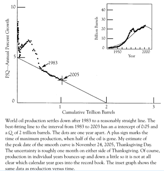
Deffeyes’s Maltheisan proof went like this: take a year-by year history of the rate of production, P and divide this by the amount of oil known to be recoverable in that year, Q. Plot this P/Q data against Q, and you find the data follows a reasonably straight line: P/Q = b-mQ. This occurs between 1962 and 1983, or between 1983 and 2005. Fro whichever straight line you pick, m and b are positive. Once you find values for m and b that you trust, you can rearrange the equation to read,

P = -mQ2+ bQ

You the calculate the peak of production from this as the point where dP/dQ = 0. With a little calculus you’ll see this occurs at Q = b/2m, or at P/Q = b/2. This is the half-way point on the P/Q vs Q line. If you extrapolate the line to zero production, P=0, you predict a total possible oil production, QT = b/m. According to this model this is always double the total Q discovered by the peak. In 1983, QT was calculated to be 1 trillion barrels. By May of 2005, again predicted to be a peak year, QT had grown to two trillion barrels.

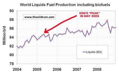
I suppose Deffayes might have suspected there was a mistake somewhere in the calculation from the way that QT had doubled, but he did not. See him lecture here in May 2005; he predicts war, famine, and pestilence, with no real chance of salvation. It’s a depressing conclusion, confidently presented by someone enamored of his own theories. In retrospect, I’d say he did not realize that he was over-enamored of his own theory, and blind to the possibility that the P/Q vs Q line might curve upward, have a positive second derivative.

Aside from his theory of peak oil, Deffayes also had a theory of oil price, one that was not all that popular. It’s not presented in the YouTube video, nor in his popular books, but it’s one that I still find valuable, and plausibly true. Deffeyes claimed the wildly varying prices of the time were the result of an inherent quay imbalance between a varying supply and an inelastic demand. If this was the cause, we’d expect the price jumps of oil up and down will match the way the wait-line at a barber shop gets longer and shorter. Assume supply varies because discoveries came in random packets, while demand rises steadily, and it all makes sense. After each new discovery, price is seen to fall. It then rises slowly till the next discovery. Price is seen as a symptom of supply unpredictability rather than a useful corrective to supply needs. This view is the opposite of Adam Smith, but I think he’s not wrong, at least in the short term with a necessary commodity like oil.

Academics accepted the peak oil prediction, I suspect, in part because it supported a Marxian remedy. If oil was running out and the market was broken, then our only recourse was government management of energy production and use. By the late 70s, Jimmy Carter told us to turn our thermostats to 65. This went with price controls, gas rationing, and a 55 mph speed limit, and a strong message of population management – birth control. We were running out of energy, we were told because we had too many people and they (we) were using too much. America’s grown days were behind us, and only the best and the brightest could be trusted to manage our decline into the abyss. I half believed these scary predictions, in part because everyone did, and in part because they made my research at Princeton particularly important. The Science fiction of the day told tales of bold energy leaders, and I was ready to step up and lead, or so I thought.

By 2009 Dr. Deffayes was being regarded as chicken little as world oil production continued to expand.

By 2009 Dr. Deffayes was being regarded as chicken little as world oil production continued to expand.

I’m happy to report that none of the dire predictions of the 70’s to 90s came to pass. Some of my colleagues became world leaders, the rest because stock brokers with their own private planes and SUVs. As of my writing in 2018, world oil production has been rising, and even King Hubbert’s original prediction of US production has been overturned. Deffayes’s reputation suffered for a few years, then politicians moved on to other dire dangers that require world-class management. Among the major dangers of today, school shootings, Ebola, and Al Gore’s claim that the ice caps will melt by 2014, flooding New York. Sooner or later, one of these predictions will come true, but the lesson I take is that it’s hard to predict change accurately.

Just when you thought US oil had beed depleted for good, production began rising. It's now higher than the 1970 peak.

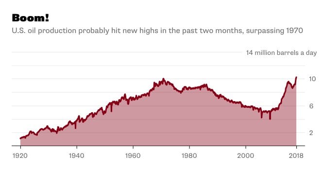
Just when you thought US oil was depleted, production began rising. We now produce more than in 1970.

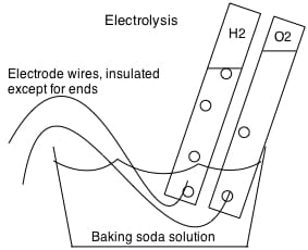
Much of the new oil production you’ll see on the chart above comes from tar-sands, oil the Deffeyes  considered unrecoverable, even while it was being recovered. We also  discovered new ways to extract leftover oil, and got better at using nuclear electricity and natural gas. In the long run, I expect nuclear electricity and hydrogen will replace oil. Trees have a value, as does solar. As for nuclear fusion, it has not turned out practical. See my analysis of why.

Robert Buxbaum, March 15, 2018. Happy Ides of March, a most republican holiday.

Why is it hot at the equator, cold at the poles?

Here’s a somewhat mathematical look at why it is hotter at the equator that at the poles. This is high school or basic college level science, using trigonometry (pre calculus), a slight step beyond the basic statement that the sun hits down more directly at the equator than at the poles. That’s the kid’s explanation, but we can understand better if we add a little math.

Solar radiation hits Detroit at an angle, as a result less radiation power hits per square meter of Detroit.

Solar radiation hits Detroit or any other non-equator point at an angle, As a result, less radiation power hits per square meter of land.

Lets use the diagram at right and trigonometry to compare the amount of sun-energy that falls on a square meter of land at the equator (0 latitude) and in a city at 42.5 N latitude (Detroit, Boston, and Rome are at this latitude). In each case, let’s consider high-noon on March 21 or September 20. These are the two equinox days, the only days each year when the day and night are equal length, and the only times when it is easy to calculate the angle of the sun as it deviates from the vertical by exactly the latitude on the days and times.

More specifically the equator is zero latitude, so on the equator at high-noon on the equinox, the sun will shine from directly overhead, or 0° from the vertical. Since the sun’s power in space is 1050 W/m2, every square meter of equator can expect to receive 1050 W of sun-energy, less the amount reflected off clouds and dust, or scattered off or air molecules (air scattering is what makes the sky blue). Further north, Detroit, Boston, and Rome sit at 42.5 latitude. At noon on March 31 the sun will strike earth at 42.5° from the vertical as shown in the lower figure above. From trigonometry, you can see that each square meter of these cities will receive cos 42.5 as much power as a square meter at the equator, except for any difference in clouds, dust, etc. Without clouds etc. that would be 1050 cos 42.5 = 774 W. Less sun power hits per square meter because each square meter is tilted. Earlier and later in the day, each spot will get less sunlight than at noon, but the proportion is the same, at least on one of the equinox days.

To calculate the likely temperature in Detroit, Boston, or Rome, I will use a simple energy balance. Ignoring heat storage in the earth for now, we will say that the heat in equals the heat out. We now ignore heat transfer by way of winds and rain, and approximate to say that the heat out leaves by black-body radiation alone, radiating into the extreme cold of space. This is not a very bad approximation since Black body radiation is the main temperature removal mechanism in most situations where large distances are involved. I’ve discussed black body radiation previously; the amount of energy radiated is proportional to luminosity, and to T4, where T is the temperature as measured in an absolute temperature scale, Kelvin or Rankin. Based on this, and assuming that the luminosity of the earth is the same in Detroit as at the equator,

T Detroit / Tequator  = √√ cos 42.5 = .927

I’ll now calculate the actual temperatures. For American convenience, I’ll choose to calculation in the Rankin Temperature scale, the absolute Fahrenheit scale. In this scale, 100°F = 560°R, 0°F = 460°R, and the temperature of space is 0°R as a good approximation. If the average temperature of the equator = 100°F = 38°C = 560°R, we calculate that the average temperature of Detroit, Boston, or Rome will be about .927 x 560 = 519°R = 59°F (15°C). This is not a bad prediction, given the assumptions. We can expect the temperature will be somewhat lower at night as there is no light, but the temperature will not fall to zero as there is retained heat from the day. The same reason, retained heat, explains why it is warmer will be warmer in these cities on September 20 than on March 31.

In the summer, these cities will be warmer because they are in the northern hemisphere, and the north pole is tilted 23°. At the height of summer (June 21) at high noon, the sun will shine on Detroit at an angle of 42.5 – 23° = 19.5° from the vertical. The difference in angle is why these cities are warmer on that day than on March 21. The equator will be cooler on that day (June 21) than on March 21 since the sun’s rays will strike the equator at 23° from the vertical on that day. These  temperature differences are behind the formation of tornadoes and hurricanes, with a tornado season in the US centering on May to July.

When looking at the poles, we find a curious problem in guessing what the average temperature will be. At noon on the equinox, the sun comes in horizontally, or at 90°from the vertical. We thus expect there is no warming power at all this day, and none for the six months of winter either. At first glance, you’d think the temperature at the poles would be zero, at least for six months of the year. It isn’t zero because there is retained heat from the summer, but still it makes for a more-difficult calculation.

To figure an average temperature of the poles, lets remember that during the 6 month summer the sun shines for 24 hours per day, and that the angle of the sun will be as high as 23° from the horizon, or 67° from the vertical for all 24 hours. Let’s assume that the retained heat from the summer is what keeps the temperature from falling too low in the winter and calculate the temperature at an .

Let’s assume that the sun comes in at the equivalent of 25° for the sun during the 6 month “day” of the polar summer. I don’t look at equinox, but rather the solar day, and note that the heating angle stays fixed through each 24 hour day during the summer, and does not decrease in the morning or as the afternoon wears on. Based on this angle, we expect that

TPole / Tequator  = √√ cos 65° = .806

TPole = .806 x 560°R = 452°R = -8°F (-22°C).

This, as it happens is 4° colder than the average temperature at the north pole, but not bad, given the assumptions. Maybe winds and water currents account for the difference. Of course there is a large temperature difference at the pole between the fall equinox and the spring equinox, but that’s to be expected. The average is, -4°F, about the temperature at night in Detroit in the winter.

One last thing, one that might be unexpected, is that temperature at the south pole is lower than at the north pole, on average -44°F. The main reason for this is that the snow on south pole is quite deep — more than 1 1/2 miles deep, with some rock underneath. As I showed elsewhere, we expect that, temperatures are lower at high altitude. Data collected from cores through the 1 1/2 mile deep snow suggest (to me) chaotic temperature change, with long ice ages, and brief (6000 year) periods of warm. The ice ages seem far worse than global warming.

Dr. Robert Buxbaum, December 30, 2017

math jokes and cartoons

uo3wgcxeParallel lines have so much in common.

It’s a shame they never get to meet.

he-who-is-without-mathematics

bad-vector-math-jokemath-for-dummies

sometimes education is the removal of false notions.

sometimes education is the removal of false notions.

pi therapy

pi therapy

Robert E. Buxbaum, January 4, 2017. Aside from the beauty of math itself, I’ve previously noted that, if your child is interested in science, the best route for development is math. I’ve also noted that Einstein did not fail at math, and that calculus is taught wrong, and probably is.

The game is rigged and you can always win.

A few months ago, I wrote a rather depressing essay based on Nobel Laureate, Kenneth Arrow’s work, and the paradox of de Condorcet. It is mathematically shown that you can not make a fair election, even if you wanted to, and no one in power wants to. The game is rigged.

To make up for that insight, I’d like to show from the work of John Forbes Nash (A Beautiful Mind) that you, personally, can win, basically all the time, if you can get someone, anyone to coöperate by trade. Let’s begin with an example in Nash’s first major paper, “The Bargaining Problem,” the one Nash is working on in the movie— read the whole paper here.  Consider two people, each with a few durable good items. Person A has a bat, a ball, a book, a whip, and a box. Person B has a pen, a toy, a knife, and a hat. Since each item is worth a different amount (has a different utility) to the owner and to the other person, there are almost always sets of trades that benefit both. In our world, where there are many people and everyone has many durable items, it is inconceivable that there are not many trades a person can make to benefit him/her while benefiting the trade partner.

Figure 3, from Nash’s, “The bargaining problem.” U1 and U2 are the utilities of the items to the two people, and O is the current state. You can improve by barter so long as your current state is not on the boundary. The parallel lines are places one could reach if money trades as well.

Good trades are even more likely when money is involved or non-durables. A person may trade his or her time for money, that is work, and any half-normal person will have enough skill to be of some value to someone. If one trades some money for durables, particularly tools, one can become rich (slowly). If one trades this work for items to make them happy (food, entertainment) they can become happier. There are just two key skills: knowing what something is worth to you, and being willing to trade. It’s not that easy for most folks to figure out what their old sofa means to them, but it’s gotten easier with garage sales and eBay.

Let us now move to the problem of elections, e.g. in this year 2016. There are few people who find the person of their dreams running for president this year. The system has fundamental flaws, and has delivered two thoroughly disliked individuals. But you can vote for a generally positive result by splitting your ticket. American society generally elects a mix of Democrats and Republicans. This mix either delivers the outcome we want, or we vote out some of the bums. Americans are generally happy with the result.

A Stamp act stamp. The British used these to tax every transaction, making it impossible for the ordinary person to benefit by small trade.

A Stamp act stamp,. Used to tax every transaction, the British made it impossible for ordinary people to benefit by small trades.

The mix does not have to involve different people, it can involve different periods of time. One can elect a Democrat president this year, and an Republican four years later. Or take the problem of time management for college students. If a student had to make a one time choice, they’d discover that you can’t have good grades, good friends, and sleep. Instead, most college students figure out you can have everything if you do one or two of these now, and switch when you get bored. And this may be the most important thing they learn.

This is my solution to Israel’s classic identity dilemma. David Ben-Gurion famously noted that Israel had the following three choices: they could be a nation of Jews living in the land of Israel, but not democratic. They could be a democratic nation in the land of Israel, but not Jewish; or they could be Jewish and democratic, but not (for the most part) in Israel. This sounds horrible until you realize that Israel can elect politicians to deliver different pairs of the options, and can have different cities that cater to thee options too. Because Jerusalem does not have to look like Tel Aviv, Israel can achieve a balance that’s better than any pure solution.

Robert E. Buxbaum, July 17-22, 2016. Balance is all, and pure solutions are a doom. I’m running for water commissioner.

if everyone agrees, something is wrong

I thought I’d try to semi-derive, and explain a remarkable mathematical paper that was published last month in The Proceedings of the Royal Society A (see full paper here). The paper demonstrates that too much agreement about a thing is counter-indicative of the thing being true. Unless an observation is blindingly obvious, near 100% agreement suggests there is a hidden flaw or conspiracy, perhaps unknown to the observers. This paper has broad application, but I thought the presentation was too confusing for most people to make use of, even those with a background in mathematics, science, or engineering. And the popular versions press versions didn’t even try to be useful. So here’s my shot:

Figure 2 from the original paper. For a method that is 80% accurate, you get your maximum reliability at the third to fifth witness. Beyond that, more agreement suggest a flaw in the people or procedure.

Figure 2 from the original paper. For a method that is 80% accurate, you get your maximum reliability at 3-5 witnesses. More agreement suggests a flaw in the people or procedure.

I will discuss only on specific application, the second one mentioned in the paper, crime (read the paper for others). Lets say there’s been a crime with several witnesses. The police line up a half-dozen, equal (?) suspects, and show them to the first witness. Lets say the first witness points to one of the suspects, the police will not arrest on this because they know that people correctly identify suspects only about 40% of the time, and incorrectly identify perhaps 10% (the say they don’t know or can’t remember the remaining 50% of time). The original paper includes the actual factions here; they’re similar. Since the witness pointed to someone, you already know he/she isn’t among the 50% who don’t know. But you don’t know if this witness is among the 40% who identify right or the 10% who identify wrong. Our confidence that this is the criminal is thus .4/(.4 +.1) = .8, or 80%.

Now you bring in the second witness. If this person identifies the same suspect, your confidence increases; to roughly (.4)2/(.42+.12) = .941,  or 94.1%. This is enough to make an arrest, but let’s say you have ten more witnesses, and all identify this same person. You might first think that this must be the guy with a confidence of (.4)10/(.410+.110) = 99.99999%, but then you wonder how unlikely it is to find ten people who identify correctly when, as we mentioned, each person has only a 40% chance. The chance of all ten witnesses identifying a suspect right is small: (.4)10 = .000104 or 0.01%. This fraction is smaller than the likelihood of having a crooked cop or a screw up the line-up (only one suspect had the right jacket, say). If crooked cops and systemic errors show up 1% of the time, and point to the correct fellow only 15% of these, we find that the chance of being right if ten out of ten agree is (0.0015 +(.4)10)/( .01+ .410+.110) = .16%. Total agreement on guilt suggests the fellow is innocent!

The graph above, the second in the paper, presents a generalization of the math I just presented: n identical tests of 80% accuracy and three different likelihoods of systemic failure. If this systemic failure rate is 1% and the chance of the error pointing right or wrong is 50/50, the chance of being right is P = (.005+ .4n)/(.01 +.4n+.1n), and is the red curve in the graph above. The authors find you get your maximum reliability when there are two to four agreeing witness.

Confidence of guilt as related to the number of judges that agree and your confidence in the integrity of the judges.

Confidence of guilt as related to the number of judges that agree and the integrity of the judges.

The Royal Society article went on to a approve of a feature of Jewish capital-punishment law. In Jewish law, capital cases are tried by 23 judges. To convict a super majority (13) must find guilty, but if all 23 judges agree on guilt the court pronounces innocent (see chart, or an anecdote about Justice Antonin Scalia). My suspicion, by the way, is that more than 1% of judges and police are crooked or inept, and that the same applies to scientific analysis of mental diseases like diagnosing ADHD or autism, and predictions about stocks or climate change. (Do 98% of scientists really agree independently?). Perhaps there are so many people in US prisons, because of excessive agreement and inaccurate witnesses, e.g Ruben Carter. I suspect the agreement on climate experts is a similar sham.

Robert Buxbaum, March 11, 2016. Here are some thoughts on how to do science right. Here is some climate data: can you spot a clear pattern of man-made change?

An approach to teaching statistics to 8th graders

There are two main obstacles students have to overcome to learn statistics: one mathematical one philosophical. The math is somewhat difficult, and will be new to a high schooler. What’s more, philosophically, it is rarely obvious what it means to discover a true pattern, or underlying cause. Nor is it obvious how to separate the general pattern from the random accident, the pattern from the variation. This philosophical confusion (cause and effect, essence and accident) is exists in the back of even in the greatest minds. Accepting and dealing with it is at the heart of the best research: seeing what is and is not captured in the formulas of the day. But it is a lot to ask of the young (or the old) who are trying to understand the statistical technique while at the same time trying to understand the subject of the statistical analysis, For young students, especially the good ones, the issue of general and specific will compound the difficulty of the experiment and of the math. Thus, I’ll try to teach statistics with a problem or two where the distinction between essential cause and random variation is uncommonly clear.

A good case to get around the philosophical issue is gambling with crooked dice. I show the class a pair of normal-looking dice and a caliper and demonstrate that the dice are not square; virtually every store-bought die is not square, so finding an uneven pair is easy. After checking my caliper, students will readily accept that these dice are crooked, and so someone who knows how it is crooked will have an unfair advantage. After enough throws, someone who knows the degree of crookedness will win more often than those who do not. Students will also accept that there is a degree of randomness in the throw, so that any pair of dice will look pretty fair if you don’t gable with them too long. I can then use statistics to see which faces show up most, and justify the whole study of statistics to deal with a world where the dice are loaded by God, and you don’t have a caliper, or any more-direct way of checking them. The underlying uneven-ness of the dice is the underlying pattern, the random part in this case is in the throw, and you want to use statistics to grasp them both.

Two important numbers to understand when trying to use statistics are the average and the standard deviation. For an honest pair of dice, you’d expect an average of 1/6 = 0.1667 for every number on the face. But throw a die a thousand times and you’ll find that hardly any of the faces show up at the average rate of 1/6. The average of all the averages will still be 1/6. We will call that grand average, 1/6 = x°-bar, and we will call the specific face average of the face Xi-bar. where i is one, two three, four, five, or six.

There is also a standard deviation — SD. This relates to how often do you expect one fact to turn up more than the next. SD = √SD2, and SD2 is defined by the following formula

SD2 = 1/n ∑(xi – x°-bar)2

Let’s pick some face of the dice, 3 say. I’ll give a value of 1 if we throw that number and 0 if we do not. For an honest pair of dice, x°-bar = 1/6, that is to say, 1 out of 6 throws will be land on the number 3, going us a value of 1, and the others won’t. In this situation, SD2 = 1/n ∑(xi – x°-bar)2 will equal 1/6 ( (1/6)2 + 5 (5/6)2 )= 1/6 (126/36) = 3.5/6 = .58333. Taking the square root, SD = 0.734. We now calculate the standard error. For honest dice, you expect that for every face, on average

SE = Xi-bar minus x°-bar = ± SD √(1/n).

By the time you’ve thrown 10,000 throws, √(1/n) = 1/100 and you expect an error on the order of 0.0073. This is to say that you expect to see each face show up between about 0.1740 and 0.1594. In point of fact, you will likely find that at least one face of your dice shows up a lot more often than this, or a lot less often. To the extent you see that, this is the extent that your dice is crooked. If you throw someone’s dice enough, you can find out how crooked they are, and you can then use this information to beat the house. That, more or less is the purpose of science, by the way: you want to beat the house — you want to live a life where you do better than you would by random chance.

As a less-mathematical way to look at the same thing — understanding statistics — I suggest we consider a crooked coin throw with only two outcomes, heads and tails. Not that I have a crooked coin, but your job as before is to figure out if the coin is crooked, and if so how crooked. This problem also appears in political polling before a major election: how do you figure out who will win between Mr Head and Ms Tail from a sampling of only a few voters. For an honest coin or an even election, on each throw, there is a 50-50 chance of head, or of Mr Head. If you do it twice, there is a 25% chance of two heads, a 25% chance of throwing two tails and a 50% chance of one of each. That’s because there are four possibilities and two ways of getting a Head and a Tail.

pascal's triangle

Pascal’s triangle

You can systematize this with a Pascal’s triangle, shown at left. Pascal’s triangle shows the various outcomes for a coin toss, and shows the ways they can be arrived at. Thus, for example, we see that, by the time you’ve thrown the coin 6 times, or polled 6 people, you’ve introduced 26 = 64 distinct outcomes, of which 20 (about 1/3) are the expected, even result: 3 heads and 3 tails. There is only 1 way to get all heads and one way to get all tails. While an honest coin is unlikely to come up all heads or tails after six throws, more often than not an honest coin will not come up with half heads. In the case above, 44 out of 64 possible outcomes describe situations with more heads than tales, or more tales than heads — with an honest coin.

Similarly, in a poll of an even election, the result will not likely come up even. This is something that confuses many political savants. The lack of an even result after relatively few throws (or phone calls) should not be used to convince us that the die is crooked, or the election has a clear winner. On the other hand there is only a 1/32 chance of getting all heads or all tails (2/64). If you call 6 people, and all claim to be for Mr Head, it is likely that Mr Head is the true favorite to a confidence of 3% = 1/32. In sports, it’s not uncommon for one side to win 6 out of 6 times. If that happens, it is a good possibility that there is a real underlying cause, e.g. that one team is really better than the other.

And now we get to how significant is significant. If you threw 4 heads and 2 tails out of 6 throws we can accept that this is not significant because there are 15 ways to get this outcome (or 30 if you also include 2 heads and 4 tail) and only 20 to get the even outcome of 3-3. But what about if you threw 5 heads and one tail? In that case the ratio is 6/20 and the odds of this being significant is better, similarly, if you called potential voters and found 5 Head supporters and 1 for Tail. What do you do? I would like to suggest you take the ratio as 12/20 — the ratio of both ways to get to this outcome to that of the greatest probability. Since 12/20 = 60%, you could say there is a 60% chance that this result is random, and a 40% chance of significance. What statisticians call this is “suggestive” at slightly over 1 standard deviation. A standard deviation, also known as σ (sigma) is a minimal standard of significance, it’s if the one tailed value is 1/2 of the most likely value. In this case, where 6 tosses come in as 5 and 1, we find the ratio to be 6/20. Since 6/20 is less than 1/2, we meet this, very minimal standard for “suggestive.” A more normative standard is when the value is 5%. Clearly 6/20 does not meet that standard, but 1/20 does; for you to conclude that the dice is likely fixed after only 6 throws, all 6 have to come up heads or tails.

From skdz. It's typical in science to say that <5% chances, p <.050 are significant. If things don't quite come out that way, you redo.

From xkcd. It’s typical in science to say that <5% chances, p< .05. If things don’t quite come out that way, you redo.

If you graph the possibilities from a large Poisson Triangle they will resemble a bell curve; in many real cases (not all) your experiential data variation will also resemble this bell curve. From a larger Poisson’s triange, or a large bell curve, you  will find that the 5% value occurs at about σ =2, that is at about twice the distance from the average as to where σ  = 1. Generally speaking, the number of observations you need is proportional to the square of the difference you are looking for. Thus, if you think there is a one-headed coin in use, it will only take 6 or seven observations; if you think the die is loaded by 10% it will take some 600 throws of that side to show it.

In many (most) experiments, you can not easily use the poisson triangle to get sigma, σ. Thus, for example, if you want to see if 8th graders are taller than 7th graders, you might measure the height of people in both classes and take an average of all the heights  but you might wonder what sigma is so you can tell if the difference is significant, or just random variation. The classic mathematical approach is to calculate sigma as the square root of the average of the square of the difference of the data from the average. Thus if the average is <h> = ∑h/N where h is the height of a student and N is the number of students, we can say that σ = √ (∑ (<h> – h)2/N). This formula is found in most books. Significance is either specified as 2 sigma, or some close variation. As convenient as this is, my preference is for this graphical version. It also show if the data is normal — an important consideration.

If you find the data is not normal, you may decide to break the data into sub-groups. E.g. if you look at heights of 7th and 8th graders and you find a lack of normal distribution, you may find you’re better off looking at the heights of the girls and boys separately. You can then compare those two subgroups to see if, perhaps, only the boys are still growing, or only the girls. One should not pick a hypothesis and then test it but collect the data first and let the data determine the analysis. This was the method of Sherlock Homes — a very worthwhile read.

Another good trick for statistics is to use a linear regression, If you are trying to show that music helps to improve concentration, try to see if more music improves it more, You want to find a linear relationship, or at lest a plausible curve relationship. Generally there is a relationship if (y – <y>)/(x-<x>) is 0.9 or so. A discredited study where the author did not use regressions, but should have, and did not report sub-groups, but should have, involved cancer and genetically modified foods. The author found cancer increased with one sub-group, and publicized that finding, but didn’t mention that cancer didn’t increase in nearby sub-groups of different doses, and decreased in a nearby sub-group. By not including the subgroups, and not doing a regression, the author mislead people for 2 years– perhaps out of a misguided attempt to help. Don’t do that.

Dr. Robert E. Buxbaum, June 5-7, 2015. Lack of trust in statistics, or of understanding of statistical formulas should not be taken as a sign of stupidity, or a symptom of ADHD. A fine book on the misuse of statistics and its pitfalls is called “How to Lie with Statistics.” Most of the examples come from advertising.

Zombie invasion model for surviving plagues

Imagine a highly infectious, people-borne plague for which there is no immunization or ready cure, e.g. leprosy or small pox in the 1800s, or bubonic plague in the 1500s assuming that the carrier was fleas on people (there is a good argument that people-fleas were the carrier, not rat-fleas). We’ll call these plagues zombie invasions to highlight understanding that there is no way to cure these diseases or protect from them aside from quarantining the infected or killing them. Classical leprosy was treated by quarantine.

I propose to model the progress of these plagues to know how to survive one, if it should arise. I will follow a recent paper out of Cornell that highlighted a fact, perhaps forgotten in the 21 century, that population density makes a tremendous difference in the rate of plague-spread. In medieval Europe plagues spread fastest in the cities because a city dweller interacted with far more people per day. I’ll attempt to simplify the mathematics of that paper without losing any of the key insights. As often happens when I try this, I’ve found a new insight.

Assume that the density of zombies per square mile is Z, and the density of susceptible people is S in the same units, susceptible population per square mile. We define a bite transmission likelihood, ß so that dS/dt = -ßSZ. The total rate of susceptibles becoming zombies is proportional to the product of the density of zombies and of susceptibles. Assume, for now, that the plague moves fast enough that we can ignore natural death, immunity, or the birth rate of new susceptibles. I’ll relax this assumption at the end of the essay.

The rate of zombie increase will be less than the rate of susceptible population decrease because some zombies will be killed or rounded up. Classically, zombies are killed by shot-gun fire to the head, by flame-throwers, or removed to leper colonies. However zombies are removed, the process requires people. We can say that, dR/dt = kSZ where R is the density per square mile of removed zombies, and k is the rate factor for killing or quarantining them. From the above, dZ/dt = (ß-k) SZ.

We now have three, non-linear, indefinite differential equations. As a first step to solving them, we set the derivates to zero and calculate the end result of the plague: what happens at t –> ∞. Using just equation 1 and setting dS/dt= 0 we see that, since ß≠0, the end result is SZ =0. Thus, there are only two possible end-outcomes: either S=0 and we’ve all become zombies or Z=0, and all the zombies are all dead or rounded up. Zombie plagues can never end in mixed live-and-let-live situations. Worse yet, rounded up zombies are dangerous.

If you start with a small fraction of infected people Z0/S0 <<1, the equations above suggest that the outcome depends entirely on k/ß. If zombies are killed/ rounded up faster than they infect/bite, all is well. Otherwise, all is zombies. A situation like this is shown in the diagram below for a population of 200 and k/ß = .6

FIG. 1. Example dynamics for progress of a normal disease and a zombie apocalypse for an initial population of 199 unin- fected and 1 infected. The S, Z, and R populations are shown in (blue, red, black respectively, with solid lines for the zombie apocalypse, and lighter lines for the normal plague. t= tNß where N is the total popula- tion. For both models the k/ß = 0.6 to show similar evolutions. In the SZR case, the S population disap- pears, while the SIR is self limiting, and only a fraction of the population becomes infected.

Fig. 1, Dynamics of a normal plague (light lines) and a zombie apocalypse (dark) for 199 uninfected and 1 infected. The S and R populations are shown in blue and black respectively. Zombie and infected populations, Z and I , are shown in red; k/ß = 0.6 and τ = tNß. With zombies, the S population disappears. With normal infection, the infected die and some S survive.

Sorry to say, things get worse for higher initial ratios,  Z0/S0 >> 0. For these cases, you can kill zombies faster than they infect you, and the last susceptible person will still be infected before the last zombie is killed. To analyze this, we create a new parameter P = Z + (1 – k/ß)S and note that dP/dt = 0 for all S and Z; the path of possible outcomes will always be along a path of constant P. We already know that, for any zombies to survive, S = 0. We now use algebra to show that the final concentration of zombies will be Z = Z0 + (1-k/ß)S0. Free zombies survive so long as the following ratio is non zero: Z0/S0 + 1- k/ß. If Z0/S0 = 1, a situation that could arise if a small army of zombies breaks out of quarantine, you’ll need a high kill ratio, k/ß > 2 or the zombies take over. It’s seen to be harder to stop a zombie outbreak than to stop the original plague. This is a strong motivation to kill any infected people you’ve rounded up, a moral dilemma that appears some plague literature.

Figure 1, from the Cornell paper, gives a sense of the time necessary to reach the final state of S=0 or Z=0. For k/ß of .6, we see that it takes is a dimensionless time τ of 25 or to reach this final, steady state of all zombies. Here, τ= t Nß and N is the total population; it takes more real time to reach τ= 25 if N is high than if N is low. We find that the best course in a zombie invasion is to head for the country hoping to find a place where N is vanishingly low, or (better yet) where Z0 is zero. This was the main conclusion of the Cornell paper.

Figure 1 also shows the progress of a more normal disease, one where a significant fraction of the infected die on their own or develop a natural immunity and recover. As before, S is the density of the susceptible, R is the density of the removed + recovered, but here I is the density of those Infected by non-zombie disease. The time-scales are the same, but the outcome is different. As before, τ = 25 but now the infected are entirely killed off or isolated, I =0 though ß > k. Some non-infected, susceptible individuals survive as well.

From this observation, I now add a new conclusion, not from the Cornell paper. It seems clear that more immune people will be in the cities. I’ve also noted that τ = 25 will be reached faster in the cities, where N is large, than in the country where N is small. I conclude that, while you will be worse off in the city at the beginning of a plague, you’re likely better off there at the end. You may need to get through an intermediate zombie zone, and you will want to get the infected to bury their own, but my new insight is that you’ll want to return to the city at the end of the plague and look for the immune remnant. This is a typical zombie story-line; it should be the winning strategy if a plague strikes too. Good luck.

Robert Buxbaum, April 21, 2015. While everything I presented above was done with differential calculus, the original paper showed a more-complete, stochastic solution. I’ve noted before that difference calculus is better. Stochastic calculus shows that, if you start with only one or two zombies, there is still a chance to survive even if ß/k is high and there is no immunity. You’ve just got to kill all the zombies early on (gun ownership can help). Here’s my statistical way to look at this. James Sethna, lead author of the Cornell paper, was one of the brightest of my Princeton PhD chums.

Brass monkey cold

In case it should ever come up in conversation, only the picture at left shows a brass monkey. The other is a bronze statue of some sort of a primate. A brass monkey is a rack used to stack cannon balls into a face centered pyramid. A cannon crew could fire about once per minute, and an engagement could last 5 hours, so you could hope to go through a lot of cannon balls during an engagement (assuming you survived).

A brass monkey cannonball holder. The classic monkeys were 10 x 10 and made of navy brass.

Small brass monkey. The classic monkey might have 9 x 9 or 10×10 cannon balls on the lower level.

Bronze sculpture of a primate playing with balls -- but look what the balls are sitting on: it's a surreal joke.

Bronze sculpture of a primate playing with balls — but look what the balls are sitting on: it’s a dada art joke.

But brass monkeys typically show up in conversation in terms of it being cold enough to freeze the balls off of a brass monkey, and if you imagine an ornamental statue, you’d never guess how cold could that be. Well, for a cannonball holder, the answer has to do with the thermal expansion of metals. Cannon balls were made of iron and the classic brass monkey was made of brass, an alloy with a much-greater thermal expansion than iron. As the temperature drops, the brass monkey contracts more than the iron balls. When the drop is enough the balls will fall off and roll around.

The thermal expansion coefficient of brass is 18.9 x 10⁻⁶/°C while the thermal expansion coefficient of iron is 11.7 x10⁻⁶/°C. The difference is 7.2×10⁻⁶/°C; this will determine the key temperature. Now consider a large brass monkey, one with 400 x 400 holes on the lower level, 399 x 399 at the second, and so on. Though it doesn’t affect the result, we’ll consider a monkey that holds 12 lb cannon balls, a typical size of 1750 -1830. Each 12 lb ball is 4.4″ in diameter at room temperature, 20°C in those days. At 20°C, this monkey is about 1760″ wide. The balls will fall off when the monkey shrinks more than the balls by about 1/3 of a diameter, 1.5″.

We can calculate ∆T, the temperature change, °C, that is required to lower the width-difference by 1.5″ as follows:

kepler conjecture, brass monkey

-1.5″ = ∆T x 1760″ x 7.2 x10⁻⁶

We find that ∆T = -118°C. The temperature where this happens is 118 degrees cooler than 20°C, or -98°C. That’s a temperature that you could, perhaps reach on the South Pole or maybe deepest Russia. It’s not likely to be a problem, especially with a smaller brass monkey.

Robert E. Buxbaum, February 21, 2015 (modified Apr. 28, 2021). Some fun thoughts: Convince yourself that the key temperature is independent of the size of the cannon balls. That is, that I didn’t need to choose 12 pounders. A bit more advanced, what is the equation for the number of balls on any particular base-size monkey. Show that the packing density is no more efficient if the bottom lawyer were an equilateral triangle, and not a square. If you liked this, you might want to know how much wood a woodchuck chucks if a woodchuck could chuck wood, or on the relationship between mustaches and WWII diplomacy.

Einstein failed high-school math –not.

I don’t know quite why people persist in claiming that Einstein failed high school math. Perhaps it’s to put down teachers –who clearly can’t teach or recognize genius — or perhaps to stake a claim to a higher understanding that’s masked by ADHD — a disease Einstein is supposed to have had. But, sorry to say, it ain’t true. Here’s Einstein’s diploma, 1896. His math and physics scores are perfect. Only his English seems to have been lacking. He would have been 17 at the time.

Einstein's high school diploma

Albert Einstein’s high school diploma, 1896.

Robert Buxbaum, December 16, 2014. Here’s Einstein relaxing in Princeton. Here’s something on black holes, and on High School calculus for non-continuous functions.

Toxic electrochemistry and biology at home

A few weeks back, I decided to do something about the low quality of experiments in modern chemistry and science sets; I posted to this blog some interesting science experiments, and some more-interesting experiments that could be done at home using the toxic (poisonous dangerous) chemicals available under the sink or on the hardware store. Here are some more. As previously, the chemicals are toxic and dangerous but available. As previously, these experiments should be done only with parental (adult) supervision. Some of these next experiments involve some math, as key aspect of science; others involve some new equipment as well as the stuff you used previously. To do them all, you will want a stop watch, a volt-amp meter, and a small transformer, available at RadioShack; you’ll also want some test tubes or similar, clear cigar tubes, wire and baking soda; for the coating experiment you’ll want copper drain clear, or copper containing fertilizer and some washers available at the hardware store; for metal casting experiment you’ll need a tin can, pliers, a gas stove and some pennies, plus a mold, some sand, good shoes, and a floor cover; and for the biology experiment you will need several 9 V batteries, and you will have to get a frog and kill it. You can skip any of these experiments, if you like and do the others. If you have not done the previous experiments, look them over or do them now.

1) The first experiments aim to add some numerical observations to our previous studies of electrolysis. Here is where you will see why we think that molecules like water are made of fixed compositions of atoms. Lets redo the water electrolysis experiment now with an Ammeter in line between the battery and one of the electrodes. With the ammeter connected, put both electrodes deep into a solution of water with a little lye, and then (while watching the ammeter) lift one electrode half out, place it back, and lift the other. You will find, I think, that one of the other electrode is the limiting electrode, and that the amperage goes to 1/2 its previous value when this electrode is half lifted. Lifting the other electrode changes neither the amperage or the amount of bubbles, but lifting this limiting electrode changes both the amount of bubbles and the amperage. If you watch closely, though, you’ll see it changes the amount of bubbles at both electrodes in proportion, and that the amount of bubbles is in promotion to the amperage. If you collect the two gasses simultaneously, you’ll see that the volume of gas collected is always in a ratio of 2 to 1. For other electrolysis (H2 and Cl2) it will be 1 to1; it’s always a ratio of small numbers. See diagram below on how to make and collect oxygen and hydrogen simultaneously by electrolyzing water with lye or baking soda as electrolyte. With lye or baking soda, you’ll find that there is always twice as much hydrogen produced as oxygen — exactly.

You can also do electrolysis with table salt or muriatic acid as an electrolyte, but for this you’ll need carbon or platinum electrodes. If you do it right, you’ll get hydrogen and chlorine, a green gas that smells bad. If you don’t do this right, using a wire instead of a carbon or platinum electrode, you’ll still get hydrogen, but no chlorine. Instead of chlorine, you’ll corrode the wire on that end, making e.g. copper chloride. With a carbon electrode and any chloride compound as the electrolyte, you’ll produce chlorine; without a chloride electrolyte, you will not produce chlorine at any voltage, or with any electrode. And if you make chlorine and check the volumes, you’ll find you always make one volume of chlorine for every volume of hydrogen. We imagine from this that the compounds are made of fixed atoms that transfer electrons in fixed whole numbers per molecule. You always make two volumes of hydrogen for every volume of oxygen because (we think) making oxygen requires twice as many electrons as making hydrogen.

At home electrolysis experiment

At home electrolysis experiment

We get the same volume of chlorine as hydrogen because making chlorine and hydrogen requires the same amount of electrons to be transferred. These are the sort of experiments that caused people to believe in atoms and molecules as the fundamental unchanging components of matter. Different solutes, voltages, and electrodes will affect how fast you make hydrogen and oxygen, as will the amount of dissolved solute, but the gas produced are always the same, and the ratio of volumes is always proportional to the amperage in a fixed ratio of small whole numbers.

As always, don’t let significant quantities of use hydrogen and oxygen or pure hydrogen and chlorine mix in a closed space. Hydrogen and oxygen is quite explosive brown’s gas; hydrogen and chlorine are reactive as well. When working with chlorine it is best to work outside or near an open window: chlorine is a poison gas.

You may also want to try this with non-electrolytes, pure water or water with sugar or alcohol dissolved. You will find there is hardly any amperage or gas with these, but the small amount of gas produced will retain the same ratio. For college level folks, here is some physics/math relating to the minimum voltage and relating to the quantities you should expect at any amperage.

2) Now let’s try electro-plating metals. Using the right solutes, metals can be made to coat your electrodes the same way that bubbles of gas coated your electrodes in the experiments above. The key is to find the right chemical, and as a start let me suggest the copper sulphate sold in hardware stores to stop root growth. As an alternative copper sulphate is often sold as part of a fertilizer solution like “Miracle grow.” Look for copper on the label, or for a blue color fertilizer. Make a solution of copper using enough copper so that the solution is recognizably green, Use two steel washers as electrodes (that is connect the wires from your battery to the washers) and put them in the solution. You will find that one side turns red, as it is coated with copper. Depending on what else your copper solution contained, bubbles may appear at the other washer, or the other washer will corrode. 

You are now ready to take this to a higher level — silver coating. take a piece of silver plated material that you want to coat, and clean it nicely with soap and water. Connect it to the electrode where you previously coated copper. Now clean out the solution carefully. Buy some silver nitrate from a drug store, and dissolve a few grams (1/8 tsp for a start) in pure water; place the silverware and the same electrodes as before, connected to the battery. For a nicer coat use a 1 1/2 volt lantern battery; the 6 V battery will work too, but the silver won’t look as nice. With silver nitrate, you’ll notice that one electrode produces gas (oxygen) and the other turns silvery. Now disconnect the silvery electrode. You can use this method to silver coat a ring, fork, or cup — anything you want to have silver coated. This process is called electroplating. As with hydrogen production, there is a proportional relationship between the time, the amperage and the amount of metal you deposit — until all the silver nitrate in solution is used up.

As a yet-more complex version, you can also electroplate without using a battery. This was my Simple electroplating (presented previously). Consider this only after you understand most everything else I’ve done. When I saw this the first time in high school I was confused.

3) Casting metal objects using melted pennies, heat from a gas stove, and sand or plaster as a cast. This is pretty easy, but sort of dangerous — you need parents help, if only as a watcher. This is a version of an experiment I did as a kid.  I did metal casting using lead that some plumbers had left over. I melted it in a tin can on our gas stove and cast “quarters” in a plaster mold. Plumbers no longer use lead, but modern pennies are mostly zinc, and will melt about as well as my lead did. They are also much safer.

As a preparation for this experiment, get a bucket full of sand. This is where you’ll put your metal when you’re done. Now get some pennies (1970 or later), a pair of pliers, and an empty clean tin can, and a gas stove. If you like you can make a plaster mold of some small object: a ring, a 50 piece — anything you might want to cast from your pennies. With parents’ help, light your gas stove, put 5-8 pennies in the empty tin can, and hold the can over the lit gas burner using your pliers. Turn the gas to high. In a few minutes the bottom of the can will burn and become red-hot. About this point, the pennies will soften and melt into a silvery puddle. By tilting the can, you can stir the metal around (don’t get it on you!). When it looks completely melted you can pour the molten pennies into your sand bucket (carefully), or over your plaster mold (carefully). If you use a mold, you’ll get a zinc copy of whatever your mold was: jewelry, coins, etc. If you work at it, you’ll learn to make fancier and fancier casts. Adult help is welcome to avoid accidents. Once the metal solidifies, you can help cool it faster by dripping water on it from a faucet. Don’t touch it while it’s hot!

A plaster mold can be made by putting a 50¢ piece at the bottom of a paper cup, pouring plaster over the coin, and waiting for it to dry. Tear off the cup, turn the plaster over and pull out the coin; you’ve got a one-sided mold, good enough to make a one-sided coin. If you enjoy this, you can learn more about casting on Wikipedia; it’s an endeavor that only costs 4 or 5 cents per try. As a safety note: wear solid leather shoes and cover the floor near the stove with a board. If you drop the metal on the floor you’ll have a permanent burn mark on the floor and your mother will not be happy. If you drop hot metal on your you’ll have a permanent injury, and you won’t be happy. Older pennies are made of copper and will not melt. Here’s a video of someone pouring a lot of metal into an ant-hill (kills lots of ants, makes a mold of the hill).

It's often helpful to ask yourself, "what would Dr. Frankenstein do?"

It’s nice to have assistants, friends and adult help in the laboratory when you do science. Even without the castle, it’s what Dr. Frankenstein did.

4) Bringing a dead frog back to life (sort of). Make a high voltage battery of 45 to 90 V battery by attaching 5-10, 9V batteries in a daisy chain they will snap together. If you touch both exposed contacts you’ll give yourself a wicked shock. If you touch the electrodes to a newly killed frog, the frog legs will kick. This is sort of groovy. It was the inspiration for Dr. Frankenstein (at right), who then decides he could bring a person back from the dead with “more power.” Frankenstein’s monster is brought back to life this way, but ends up killing the good doctor. Shocks are sometimes helpful reanimating people stricken by heat attacks, and many buildings have shockers for this purpose. But don’t try to bring back the long-dead. By all accounts, the results are less-than pleasing. Try dissecting the rest of the frog and guess what each part is (a world book encyclopedia helps). As I recall, the heart keeps going for a while after it’s out of the frog — spooky.

5) Another version of this shocker is made with a small transformer (1″ square, say, radioshack) and a small battery (1.5-6V). Don’t use the 90V battery, you’ll kill someone. As a first version of this shocker, strip 1″ of  insulation off of the ends of some wire 12″ long say, and attach one end to two paired wires of the transformer (there will usually be a diagram in the box). If the transformer already has some wires coming out, all you have to do is strip more insulation off the ends so 1″ is un-inuslated. Take two paired ends in your hand, holding onto the uninsulated part and touch both to the battery for a second or two. Then disconnect them while holding the bare wires; you’ll get a shock. As a nastier version, get a friend to hope the opposite pair of wires on the uninsulated parts, while you hold the insulated parts of your two. Touch your two to the battery and disconnect while holding the insulation, you will see a nice spark, and your friend will get a nice shock. Play with it; different arrangements give more sparks or bigger shocks. Another thing you can do: put your experiment near a radio or TV. The transformer sparks will interfere with most nearby electronics; you can really mess up a computer this way, so keep it far from your computer. This is how wireless radio worked long ago, and how modern warfare will probably go. The atom bomb was detonated with a spark like this.

If you want to do more advanced science, it’s a good idea to learn math. This is important for statistics, for engineering, for quantum mechanics, and can even help for music. Get a few good high school or college books and read them cover to cover. An approach to science is to try to make something cool, that sort-of works, and then try to improve it. You then decide what a better version would work like,  modify your original semi-randomly and see if you’re going in the right direction. Don’t redesign with only one approach –it may not work. Read whatever you can, but don’t believe all you read. Often books are misleading, or wrong, and blogs are worse (I ought to know). When you find mistakes, note them in the margin, and try to explain them. You may find you were right, or that the book was right, but it’s a learning experience. If you like you can write the author and inform him/her of the errors. I find mailed letters are more respectful than e-mails — it shows you put in more effort.

Robert Buxbaum, February 20, 2014. Here’s the difference between metals and non-metals, and a periodic table cup that I made, and sell. And here’s a difference between science and religion – reproducibility.