Category Archives: math

An approach to teaching statistics to 8th graders

There are two main obstacles students have to overcome to learn statistics: one mathematical one philosophical. The math is somewhat difficult, and will be new to a high schooler. What’s more, philosophically, it is rarely obvious what it means to discover a true pattern, or underlying cause. Nor is it obvious how to separate the general pattern from the random accident, the pattern from the variation. This philosophical confusion (cause and effect, essence and accident) is exists in the back of even in the greatest minds. Accepting and dealing with it is at the heart of the best research: seeing what is and is not captured in the formulas of the day. But it is a lot to ask of the young (or the old) who are trying to understand the statistical technique while at the same time trying to understand the subject of the statistical analysis, For young students, especially the good ones, the issue of general and specific will compound the difficulty of the experiment and of the math. Thus, I’ll try to teach statistics with a problem or two where the distinction between essential cause and random variation is uncommonly clear.

A good case to get around the philosophical issue is gambling with crooked dice. I show the class a pair of normal-looking dice and a caliper and demonstrate that the dice are not square; virtually every store-bought die is not square, so finding an uneven pair is easy. After checking my caliper, students will readily accept that these dice are crooked, and so someone who knows how it is crooked will have an unfair advantage. After enough throws, someone who knows the degree of crookedness will win more often than those who do not. Students will also accept that there is a degree of randomness in the throw, so that any pair of dice will look pretty fair if you don’t gable with them too long. I can then use statistics to see which faces show up most, and justify the whole study of statistics to deal with a world where the dice are loaded by God, and you don’t have a caliper, or any more-direct way of checking them. The underlying uneven-ness of the dice is the underlying pattern, the random part in this case is in the throw, and you want to use statistics to grasp them both.

Two important numbers to understand when trying to use statistics are the average and the standard deviation. For an honest pair of dice, you’d expect an average of 1/6 = 0.1667 for every number on the face. But throw a die a thousand times and you’ll find that hardly any of the faces show up at the average rate of 1/6. The average of all the averages will still be 1/6. We will call that grand average, 1/6 = x°-bar, and we will call the specific face average of the face Xi-bar. where i is one, two three, four, five, or six.

There is also a standard deviation — SD. This relates to how often do you expect one fact to turn up more than the next. SD = √SD2, and SD2 is defined by the following formula

SD2 = 1/n ∑(xi – x°-bar)2

Let’s pick some face of the dice, 3 say. I’ll give a value of 1 if we throw that number and 0 if we do not. For an honest pair of dice, x°-bar = 1/6, that is to say, 1 out of 6 throws will be land on the number 3, going us a value of 1, and the others won’t. In this situation, SD2 = 1/n ∑(xi – x°-bar)2 will equal 1/6 ( (1/6)2 + 5 (5/6)2 )= 1/6 (126/36) = 3.5/6 = .58333. Taking the square root, SD = 0.734. We now calculate the standard error. For honest dice, you expect that for every face, on average

SE = Xi-bar minus x°-bar = ± SD √(1/n).

By the time you’ve thrown 10,000 throws, √(1/n) = 1/100 and you expect an error on the order of 0.0073. This is to say that you expect to see each face show up between about 0.1740 and 0.1594. In point of fact, you will likely find that at least one face of your dice shows up a lot more often than this, or a lot less often. To the extent you see that, this is the extent that your dice is crooked. If you throw someone’s dice enough, you can find out how crooked they are, and you can then use this information to beat the house. That, more or less is the purpose of science, by the way: you want to beat the house — you want to live a life where you do better than you would by random chance.

As a less-mathematical way to look at the same thing — understanding statistics — I suggest we consider a crooked coin throw with only two outcomes, heads and tails. Not that I have a crooked coin, but your job as before is to figure out if the coin is crooked, and if so how crooked. This problem also appears in political polling before a major election: how do you figure out who will win between Mr Head and Ms Tail from a sampling of only a few voters. For an honest coin or an even election, on each throw, there is a 50-50 chance of head, or of Mr Head. If you do it twice, there is a 25% chance of two heads, a 25% chance of throwing two tails and a 50% chance of one of each. That’s because there are four possibilities and two ways of getting a Head and a Tail.

pascal's triangle

Pascal’s triangle

You can systematize this with a Pascal’s triangle, shown at left. Pascal’s triangle shows the various outcomes for a coin toss, and shows the ways they can be arrived at. Thus, for example, we see that, by the time you’ve thrown the coin 6 times, or polled 6 people, you’ve introduced 26 = 64 distinct outcomes, of which 20 (about 1/3) are the expected, even result: 3 heads and 3 tails. There is only 1 way to get all heads and one way to get all tails. While an honest coin is unlikely to come up all heads or tails after six throws, more often than not an honest coin will not come up with half heads. In the case above, 44 out of 64 possible outcomes describe situations with more heads than tales, or more tales than heads — with an honest coin.

Similarly, in a poll of an even election, the result will not likely come up even. This is something that confuses many political savants. The lack of an even result after relatively few throws (or phone calls) should not be used to convince us that the die is crooked, or the election has a clear winner. On the other hand there is only a 1/32 chance of getting all heads or all tails (2/64). If you call 6 people, and all claim to be for Mr Head, it is likely that Mr Head is the true favorite to a confidence of 3% = 1/32. In sports, it’s not uncommon for one side to win 6 out of 6 times. If that happens, it is a good possibility that there is a real underlying cause, e.g. that one team is really better than the other.

And now we get to how significant is significant. If you threw 4 heads and 2 tails out of 6 throws we can accept that this is not significant because there are 15 ways to get this outcome (or 30 if you also include 2 heads and 4 tail) and only 20 to get the even outcome of 3-3. But what about if you threw 5 heads and one tail? In that case the ratio is 6/20 and the odds of this being significant is better, similarly, if you called potential voters and found 5 Head supporters and 1 for Tail. What do you do? I would like to suggest you take the ratio as 12/20 — the ratio of both ways to get to this outcome to that of the greatest probability. Since 12/20 = 60%, you could say there is a 60% chance that this result is random, and a 40% chance of significance. What statisticians call this is “suggestive” at slightly over 1 standard deviation. A standard deviation, also known as σ (sigma) is a minimal standard of significance, it’s if the one tailed value is 1/2 of the most likely value. In this case, where 6 tosses come in as 5 and 1, we find the ratio to be 6/20. Since 6/20 is less than 1/2, we meet this, very minimal standard for “suggestive.” A more normative standard is when the value is 5%. Clearly 6/20 does not meet that standard, but 1/20 does; for you to conclude that the dice is likely fixed after only 6 throws, all 6 have to come up heads or tails.

From skdz. It's typical in science to say that <5% chances, p <.050 are significant. If things don't quite come out that way, you redo.

From xkcd. It’s typical in science to say that <5% chances, p< .05. If things don’t quite come out that way, you redo.

If you graph the possibilities from a large Poisson Triangle they will resemble a bell curve; in many real cases (not all) your experiential data variation will also resemble this bell curve. From a larger Poisson’s triange, or a large bell curve, you  will find that the 5% value occurs at about σ =2, that is at about twice the distance from the average as to where σ  = 1. Generally speaking, the number of observations you need is proportional to the square of the difference you are looking for. Thus, if you think there is a one-headed coin in use, it will only take 6 or seven observations; if you think the die is loaded by 10% it will take some 600 throws of that side to show it.

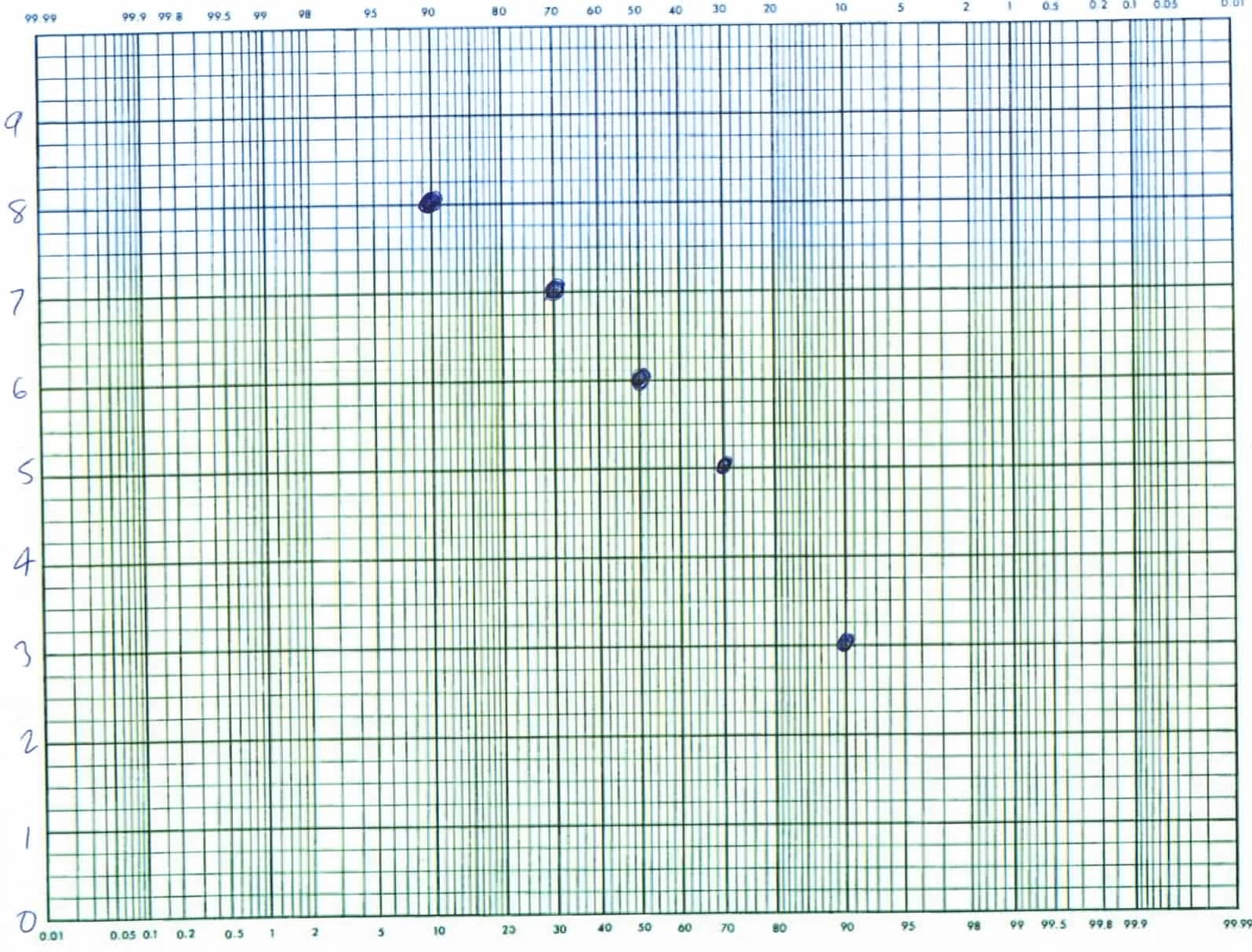
In many (most) experiments, you can not easily use the poisson triangle to get sigma, σ. Thus, for example, if you want to see if 8th graders are taller than 7th graders, you might measure the height of people in both classes and take an average of all the heights  but you might wonder what sigma is so you can tell if the difference is significant, or just random variation. The classic mathematical approach is to calculate sigma as the square root of the average of the square of the difference of the data from the average. Thus if the average is <h> = ∑h/N where h is the height of a student and N is the number of students, we can say that σ = √ (∑ (<h> – h)2/N). This formula is found in most books. Significance is either specified as 2 sigma, or some close variation. As convenient as this is, my preference is for this graphical version. It also show if the data is normal — an important consideration.

If you find the data is not normal, you may decide to break the data into sub-groups. E.g. if you look at heights of 7th and 8th graders and you find a lack of normal distribution, you may find you’re better off looking at the heights of the girls and boys separately. You can then compare those two subgroups to see if, perhaps, only the boys are still growing, or only the girls. One should not pick a hypothesis and then test it but collect the data first and let the data determine the analysis. This was the method of Sherlock Homes — a very worthwhile read.

Another good trick for statistics is to use a linear regression, If you are trying to show that music helps to improve concentration, try to see if more music improves it more, You want to find a linear relationship, or at lest a plausible curve relationship. Generally there is a relationship if (y – <y>)/(x-<x>) is 0.9 or so. A discredited study where the author did not use regressions, but should have, and did not report sub-groups, but should have, involved cancer and genetically modified foods. The author found cancer increased with one sub-group, and publicized that finding, but didn’t mention that cancer didn’t increase in nearby sub-groups of different doses, and decreased in a nearby sub-group. By not including the subgroups, and not doing a regression, the author mislead people for 2 years– perhaps out of a misguided attempt to help. Don’t do that.

Dr. Robert E. Buxbaum, June 5-7, 2015. Lack of trust in statistics, or of understanding of statistical formulas should not be taken as a sign of stupidity, or a symptom of ADHD. A fine book on the misuse of statistics and its pitfalls is called “How to Lie with Statistics.” Most of the examples come from advertising.

Zombie invasion model for surviving plagues

Imagine a highly infectious, people-borne plague for which there is no immunization or ready cure, e.g. leprosy or small pox in the 1800s, or bubonic plague in the 1500s assuming that the carrier was fleas on people (there is a good argument that people-fleas were the carrier, not rat-fleas). We’ll call these plagues zombie invasions to highlight understanding that there is no way to cure these diseases or protect from them aside from quarantining the infected or killing them. Classical leprosy was treated by quarantine.

I propose to model the progress of these plagues to know how to survive one, if it should arise. I will follow a recent paper out of Cornell that highlighted a fact, perhaps forgotten in the 21 century, that population density makes a tremendous difference in the rate of plague-spread. In medieval Europe plagues spread fastest in the cities because a city dweller interacted with far more people per day. I’ll attempt to simplify the mathematics of that paper without losing any of the key insights. As often happens when I try this, I’ve found a new insight.

Assume that the density of zombies per square mile is Z, and the density of susceptible people is S in the same units, susceptible population per square mile. We define a bite transmission likelihood, ß so that dS/dt = -ßSZ. The total rate of susceptibles becoming zombies is proportional to the product of the density of zombies and of susceptibles. Assume, for now, that the plague moves fast enough that we can ignore natural death, immunity, or the birth rate of new susceptibles. I’ll relax this assumption at the end of the essay.

The rate of zombie increase will be less than the rate of susceptible population decrease because some zombies will be killed or rounded up. Classically, zombies are killed by shot-gun fire to the head, by flame-throwers, or removed to leper colonies. However zombies are removed, the process requires people. We can say that, dR/dt = kSZ where R is the density per square mile of removed zombies, and k is the rate factor for killing or quarantining them. From the above, dZ/dt = (ß-k) SZ.

We now have three, non-linear, indefinite differential equations. As a first step to solving them, we set the derivates to zero and calculate the end result of the plague: what happens at t –> ∞. Using just equation 1 and setting dS/dt= 0 we see that, since ß≠0, the end result is SZ =0. Thus, there are only two possible end-outcomes: either S=0 and we’ve all become zombies or Z=0, and all the zombies are all dead or rounded up. Zombie plagues can never end in mixed live-and-let-live situations. Worse yet, rounded up zombies are dangerous.

If you start with a small fraction of infected people Z0/S0 <<1, the equations above suggest that the outcome depends entirely on k/ß. If zombies are killed/ rounded up faster than they infect/bite, all is well. Otherwise, all is zombies. A situation like this is shown in the diagram below for a population of 200 and k/ß = .6

FIG. 1. Example dynamics for progress of a normal disease and a zombie apocalypse for an initial population of 199 unin- fected and 1 infected. The S, Z, and R populations are shown in (blue, red, black respectively, with solid lines for the zombie apocalypse, and lighter lines for the normal plague. t= tNß where N is the total popula- tion. For both models the k/ß = 0.6 to show similar evolutions. In the SZR case, the S population disap- pears, while the SIR is self limiting, and only a fraction of the population becomes infected.

Fig. 1, Dynamics of a normal plague (light lines) and a zombie apocalypse (dark) for 199 uninfected and 1 infected. The S and R populations are shown in blue and black respectively. Zombie and infected populations, Z and I , are shown in red; k/ß = 0.6 and τ = tNß. With zombies, the S population disappears. With normal infection, the infected die and some S survive.

Sorry to say, things get worse for higher initial ratios,  Z0/S0 >> 0. For these cases, you can kill zombies faster than they infect you, and the last susceptible person will still be infected before the last zombie is killed. To analyze this, we create a new parameter P = Z + (1 – k/ß)S and note that dP/dt = 0 for all S and Z; the path of possible outcomes will always be along a path of constant P. We already know that, for any zombies to survive, S = 0. We now use algebra to show that the final concentration of zombies will be Z = Z0 + (1-k/ß)S0. Free zombies survive so long as the following ratio is non zero: Z0/S0 + 1- k/ß. If Z0/S0 = 1, a situation that could arise if a small army of zombies breaks out of quarantine, you’ll need a high kill ratio, k/ß > 2 or the zombies take over. It’s seen to be harder to stop a zombie outbreak than to stop the original plague. This is a strong motivation to kill any infected people you’ve rounded up, a moral dilemma that appears some plague literature.

Figure 1, from the Cornell paper, gives a sense of the time necessary to reach the final state of S=0 or Z=0. For k/ß of .6, we see that it takes is a dimensionless time τ of 25 or to reach this final, steady state of all zombies. Here, τ= t Nß and N is the total population; it takes more real time to reach τ= 25 if N is high than if N is low. We find that the best course in a zombie invasion is to head for the country hoping to find a place where N is vanishingly low, or (better yet) where Z0 is zero. This was the main conclusion of the Cornell paper.

Figure 1 also shows the progress of a more normal disease, one where a significant fraction of the infected die on their own or develop a natural immunity and recover. As before, S is the density of the susceptible, R is the density of the removed + recovered, but here I is the density of those Infected by non-zombie disease. The time-scales are the same, but the outcome is different. As before, τ = 25 but now the infected are entirely killed off or isolated, I =0 though ß > k. Some non-infected, susceptible individuals survive as well.

From this observation, I now add a new conclusion, not from the Cornell paper. It seems clear that more immune people will be in the cities. I’ve also noted that τ = 25 will be reached faster in the cities, where N is large, than in the country where N is small. I conclude that, while you will be worse off in the city at the beginning of a plague, you’re likely better off there at the end. You may need to get through an intermediate zombie zone, and you will want to get the infected to bury their own, but my new insight is that you’ll want to return to the city at the end of the plague and look for the immune remnant. This is a typical zombie story-line; it should be the winning strategy if a plague strikes too. Good luck.

Robert Buxbaum, April 21, 2015. While everything I presented above was done with differential calculus, the original paper showed a more-complete, stochastic solution. I’ve noted before that difference calculus is better. Stochastic calculus shows that, if you start with only one or two zombies, there is still a chance to survive even if ß/k is high and there is no immunity. You’ve just got to kill all the zombies early on (gun ownership can help). Here’s my statistical way to look at this. James Sethna, lead author of the Cornell paper, was one of the brightest of my Princeton PhD chums.

Brass monkey cold

In case it should ever come up in conversation, only the picture at left shows a brass monkey. The other is a bronze statue of some sort of a primate. A brass monkey is a rack used to stack cannon balls into a face centered pyramid. A cannon crew could fire about once per minute, and an engagement could last 5 hours, so you could hope to go through a lot of cannon balls during an engagement (assuming you survived).

A brass monkey cannonball holder. The classic monkeys were 10 x 10 and made of navy brass.

Small brass monkey. The classic monkey might have 9 x 9 or 10×10 cannon balls on the lower level.

Bronze sculpture of a primate playing with balls -- but look what the balls are sitting on: it's a surreal joke.

Bronze sculpture of a primate playing with balls — but look what the balls are sitting on: it’s a dada art joke.

But brass monkeys typically show up in conversation in terms of it being cold enough to freeze the balls off of a brass monkey, and if you imagine an ornamental statue, you’d never guess how cold could that be. Well, for a cannonball holder, the answer has to do with the thermal expansion of metals. Cannon balls were made of iron and the classic brass monkey was made of brass, an alloy with a much-greater thermal expansion than iron. As the temperature drops, the brass monkey contracts more than the iron balls. When the drop is enough the balls will fall off and roll around.

The thermal expansion coefficient of brass is 18.9 x 10⁻⁶/°C while the thermal expansion coefficient of iron is 11.7 x10⁻⁶/°C. The difference is 7.2×10⁻⁶/°C; this will determine the key temperature. Now consider a large brass monkey, one with 400 x 400 holes on the lower level, 399 x 399 at the second, and so on. Though it doesn’t affect the result, we’ll consider a monkey that holds 12 lb cannon balls, a typical size of 1750 -1830. Each 12 lb ball is 4.4″ in diameter at room temperature, 20°C in those days. At 20°C, this monkey is about 1760″ wide. The balls will fall off when the monkey shrinks more than the balls by about 1/3 of a diameter, 1.5″.

We can calculate ∆T, the temperature change, °C, that is required to lower the width-difference by 1.5″ as follows:

kepler conjecture, brass monkey

-1.5″ = ∆T x 1760″ x 7.2 x10⁻⁶

We find that ∆T = -118°C. The temperature where this happens is 118 degrees cooler than 20°C, or -98°C. That’s a temperature that you could, perhaps reach on the South Pole or maybe deepest Russia. It’s not likely to be a problem, especially with a smaller brass monkey.

Robert E. Buxbaum, February 21, 2015 (modified Apr. 28, 2021). Some fun thoughts: Convince yourself that the key temperature is independent of the size of the cannon balls. That is, that I didn’t need to choose 12 pounders. A bit more advanced, what is the equation for the number of balls on any particular base-size monkey. Show that the packing density is no more efficient if the bottom lawyer were an equilateral triangle, and not a square. If you liked this, you might want to know how much wood a woodchuck chucks if a woodchuck could chuck wood, or on the relationship between mustaches and WWII diplomacy.

Einstein failed high-school math –not.

I don’t know quite why people persist in claiming that Einstein failed high school math. Perhaps it’s to put down teachers –who clearly can’t teach or recognize genius — or perhaps to stake a claim to a higher understanding that’s masked by ADHD — a disease Einstein is supposed to have had. But, sorry to say, it ain’t true. Here’s Einstein’s diploma, 1896. His math and physics scores are perfect. Only his English seems to have been lacking. He would have been 17 at the time.

Einstein's high school diploma

Albert Einstein’s high school diploma, 1896.

Robert Buxbaum, December 16, 2014. Here’s Einstein relaxing in Princeton. Here’s something on black holes, and on High School calculus for non-continuous functions.

Patterns in climate; change is the only constant

There is a general problem when looking for climate trends: you have to look at weather data. That’s a problem because weather data goes back thousands of years, and it’s always changing. As a result it’s never clear what start year to use for the trend. If you start too early or too late the trend disappears. If you start your trend line in a hot year, like in the late roman period, the trend will show global cooling. If you start in a cold year, like the early 1970s, or the small ice age (1500 -1800) you’ll find global warming: perhaps too much. Begin 10-15 years ago, and you’ll find no change in global temperatures.

Ice coverage data shows the same problem: take the Canadian Arctic Ice maximums, shown below. If you start your regression in 1980-83, the record ice year (green) you’ll see ice loss. If you start in 1971, the year of minimum ice (red), you’ll see ice gain. It might also be nice to incorporate physics thought a computer model of the weather, but this method doesn’t seem to help. Perhaps that’s because the physics models generally have to be fed coefficients calculated from the trend line. Using the best computers and a trend line showing ice loss, the US Navy predicted, in January 2006, that the Arctic would be ice-free by 2013. It didn’t happen; a new prediction is 2016 — something I suspect is equally unlikely. Five years ago the National Academy of Sciences predicted global warming would resume in the next year or two — it didn’t either. Garbage in -garbage out, as they say.

Arctic Ice in Northern Canada waters, 1970-2014 from icecanada.ca 2014 is not totally in yet. What year do you start when looking for a trend?

Arctic Ice in Northern Canada waters, 1971-2014 from the Canadian ice service 2014 is not totally in yet , but is likely to exceed 2013. If you are looking for trends, in what year do you start?

The same trend problem appears with predicting sea temperatures and el Niño, a Christmastime warming current in the Pacific ocean. This year, 2013-14, was predicted to be a super El Niño, an exceptionally hot, stormy year with exceptionally strong sea currents. Instead, there was no el Niño, and many cities saw record cold — Detroit by 9 degrees. The Antarctic ice hit record levels, stranding a ship of anti warming activists. There were record few hurricanes.  As I look at the Pacific sea temperature from 1950 to the present, below, I see change, but no pattern or direction: El Nada (the nothing). If one did a regression analysis, the slope might be slightly positive or negative, but r squared, the significance, would be near zero. There is no real directionality, just noise if 1950 is the start date.

El Niño and La Niña since 1950. There is no sign that they are coming more often, or stronger. Nor is there evidence even that the ocean is warming.

El Niño and La Niña since 1950. There is no sign that they are coming more often, or stronger. Nor is clear evidence that the ocean is warming.

This appears to be as much a fundamental problem in applied math as in climate science: when looking for a trend, where do you start, how do you handle data confidence, and how do you prevent bias? A thought I’ve had is to try to weight a regression in terms of the confidence in the data. The Canadian ice data shows that the Canadian Ice Service is less confident about their older data than the new; this is shown by the grey lines. It would be nice if some form of this confidence could be incorporated into the regression trend analysis, but I’m not sure how to do this right.

It’s not so much that I doubt global warming, but I’d like a better explanation of the calculation. Weather changes: how do you know when you’re looking at climate, not weather? The president of the US claimed that the science is established, and Prince Charles of England claimed climate skeptics were headless chickens, but it’s certainly not predictive, and that’s the normal standard of knowledge. Neither country has any statement of how one would back up their statements. If this is global warming, I’d expect it to be warm.

Robert Buxbaum, Feb 5, 2014. Here’s a post I’ve written on the scientific method, and on dealing with abnormal statistics. I’ve also written about an important recent statistical fraud against genetically modified corn. As far as energy policy, I’m inclined to prefer hydrogen over batteries, and nuclear over wind and solar. The president has promoted the opposite policy — for unexplained, “scientific” reasons.

Fractal power laws and radioactive waste decay

Here’s a fairly simple model for nuclear reactor decay heat versus time. It’s based on a fractal model I came up with for dealing with the statistics of crime, fires, etc. The start was to notice that radioactive waste is typically a mixture of isotopes with different decay times and different decay heats. I then came to suspect that there would be a general fractal relation, and that the fractal relation would hold through as the elements of the mixed waste decayed to more stable, less radioactive products. After looking a bit, if seems that the fractal time characteristic is time to the 1/4 power, that is

heat output = H° exp (-at1/4).

Here H° is the heat output rate at some time =0 and “a” is a characteristic of the waste. Different waste mixes will have different values of this decay characteristic.

If nuclear waste consisted of one isotope and one decay path, the number of atoms decaying per day would decrease exponentially with time to the power of 1. If there were only one daughter product produced, and it were non-radioactive, the heat output of a sample would also decay with time to the power of 1. Thus, Heat output would equal  H° exp (-at) and a plot of the log of the decay heat would be linear against linear time — you could plot it all conveniently on semi-log paper.

But nuclear waste generally consists of many radioactive components with different half lives, and these commpnents decay into other radioactive isotopes, all of whom have half-lives that vary by quite a lot. The result is that a semi-log plot is rarely helpful.  Some people therefore plot radioactivity on a log-log plot, typically including a curve for each major isotope and decay mode. I find these plots hardly useful. They are certainly impossible to extrapolate. What I’d like to propose instead is a fractal variation of the original semi-log plot: a  plot of the log of the heat rate against a fractal time. As shown below the use of time to the 1/4 power seems to be helpful. The plot is similar to a fractal decay model that I’d developed for crimes and fires a few weeks ago

Afterheat of fuel rods used to generate 20 kW/kg U; Top graph 35 MW-days/kg U; bottom graph 20 Mw-day /kg  U. Data from US NRC Regulatory Guide 3.54 - Spent Fuel Heat Generation in an Independent Spent Fuel Storage Installation, rev 1, 1999. http://www.nrc.gov/reading-rm/doc-collections/reg-guides/fuels-materials/rg/03-054/

After-heat of nuclear fuel rods used at 20 kW/kg U; Top graph 35 MW-days/kg U; bottom graph 20 Mw-day /kg U. Data from US NRC Regulatory Guide 3.54. A typical reactor has 200,000 kg of uranium.

A plausible justification for this fractal semi-log plot is to observe that the half-life of daughter isotopes relates to the parent isotopes. Unless I find that someone else has come up with this sort of plot or analysis before, I’ll call it after myself: a Buxbaum Mandelbrot plot –Why not?

Nuclear power is attractive because it is a lot more energy dense than any normal fuel. Still the graph at right illustrates the problem of radioactive waste. With nuclear, you generate about 35 MW-days of power per kg of uranium. This is enough to power an average US home for 8 years, but it produces 1 kg of radioactive waste. Even after 81 years the waste is generating about 1/2 W of decay heat. It should be easier to handle and store the 1 kg of spent uranium than to deal with the many tons of coal-smoke produced when 35 MW-days of electricity is made from coal, still, there is reason to worry about the decay heat.

I’ve made a similar plot of decay heat of a fusion reactor, see below. Fusion looks better in this regard. A fission-based nuclear reactor to power 1/2 of Detroit, would hold some 200,000 kg of uranium that would be replaced every 5 years. Even 81 years after removal, the after-heat would be about 100 kW, and that’s a lot.

Afterheat of a 4000 MWth Fusion Reactor, from UMAC III Report. Nb-1%Zr is a fairly common high-temerature engineering material of construction.

After-heat of a 4000 MWth Fusion Reactor built from niobium-1%zirconium; from UWMAC III Report. The after heat is far less than with normal uranium fission.

The plot of the after-heat of a similar power fusion reactor (right) shows a far greater slope, but the same time to the1/4 power dependence. The heat output drops from 1 MW at 3 weeks to only 100 W after 1 year and far less than 1 W after 81 years. Nuclear fusion is still a few years off, but the plot at left shows the advantages fairly clearly, I. think.

This plot was really designed to look at the statistics of crime, fires, and the need for servers / checkout people.

Dr. R.E. Buxbaum, January 2, 2014, edited Aug 30, 2022. *A final, final thought about theory from Yogi Berra: “In theory, it matches reality.”

Near-Poisson statistics: how many police – firemen for a small city?

In a previous post, I dealt with the nearly-normal statistics of common things, like river crests, and explained why 100 year floods come more often than once every hundred years. As is not uncommon, the data was sort-of like a normal distribution, but deviated at the tail (the fantastic tail of the abnormal distribution). But now I’d like to present my take on a sort of statistics that (I think) should be used for the common problem of uncommon events: car crashes, fires, epidemics, wars…

Normally the mathematics used for these processes is Poisson statistics, and occasionally exponential statistics. I think these approaches lead to incorrect conclusions when applied to real-world cases of interest, e.g. choosing the size of a police force or fire department of a small town that rarely sees any crime or fire. This is relevant to Oak Park Michigan (where I live). I’ll show you how it’s treated by Poisson, and will then suggest a simpler way that’s more relevant.

First, consider an idealized version of Oak Park, Michigan (a semi-true version until the 1980s): the town had a small police department and a small fire department that saw only occasional crimes or fires, all of which required only 2 or 4 people respectively. Lets imagine that the likelihood of having one small fire at a given time is x = 5%, and that of having a violent crime is y =5% (it was 6% in 2011). A police department will need to have to have 2 policemen on call at all times, but will want 4 on the 0.25% chance that there are two simultaneous crimes (.05 x .05 = .0025); the fire department will want 8 souls on call at all times for the same reason. Either department will use the other 95% of their officers dealing with training, paperwork, investigations of less-immediate cases, care of equipment, and visiting schools, but this number on call is needed for immediate response. As there are 8760 hours per year and the police and fire workers only work 2000 hours, you’ll need at least 4.4 times this many officers. We’ll add some more for administration and sick-day relief, and predict a total staff of 20 police and 40 firemen. This is, more or less, what it was in the 1980s.

If each fire or violent crime took 3 hours (1/8 of a day), you’ll find that the entire on-call staff was busy 7.3 times per year (8x365x.0025 = 7.3), or a bit more since there is likely a seasonal effect, and since fires and violent crimes don’t fall into neat time slots. Having 3 fires or violent crimes simultaneously was very rare — and for those rare times, you could call on nearby communities, or do triage.

In response to austerity (towns always overspend in the good times, and come up short later), Oak Park realized it could use fewer employees if they combined the police and fire departments into an entity renamed “Public safety.” With 45-55 employees assigned to combined police / fire duty they’d still be able to handle the few violent crimes and fires. The sum of these events occurs 10% of the time, and we can apply the sort of statistics above to suggest that about 91% of the time there will be neither a fire nor violent crime; about 9% of the time there will be one or more fires or violent crimes (there is a 5% chance for each, but also a chance that 2 happen simultaneously). At least two events will occur 0.9% of the time (2 fires, 2 crimes or one of each), and they will have 3 or more events .09% of the time, or twice per year. The combined force allowed fewer responders since it was only rarely that 4 events happened simultaneously, and some of those were 4 crimes or 3 crimes and a fire — events that needed fewer responders. Your only real worry was when you have 3 fires, something that should happen every 3 years, or so, an acceptable risk at the time.

Before going to what caused this model of police and fire service to break down as Oak Park got bigger, I should explain Poisson statistics, exponential Statistics, and Power Law/ Fractal Statistics. The only type of statistics taught for dealing with crime like this is Poisson statistics, a type that works well when the events happen so suddenly and pass so briefly that we can claim to be interested in only how often we will see multiples of them in a period of time. The Poisson distribution formula is, P = rke/r! where P is the Probability of having some number of events, r is the total number of events divided by the total number of periods, and k is the number of events we are interested in.

Using the data above for a period-time of 3 hours, we can say that r= .1, and the likelihood of zero, one, or two events begin in the 3 hour period is 90.4%, 9.04% and 0.45%. These numbers are reasonable in terms of when events happen, but they are irrelevant to the problem anyone is really interested in: what resources are needed to come to the aid of the victims. That’s the problem with Poisson statistics: it treats something that no one cares about (when the thing start), and under-predicts the important things, like how often you’ll have multiple events in-progress. For 4 events, Poisson statistics predicts it happens only .00037% of the time — true enough, but irrelevant in terms of how often multiple teams are needed out on the job. We need four teams no matter if the 4 events began in a single 3 hour period or in close succession in two adjoining periods. The events take time to deal with, and the time overlaps.

The way I’d dealt with these events, above, suggests a power law approach. In this case, each likelihood was 1/10 the previous, and the probability P = .9 x10-k . This is called power law statistics. I’ve never seen it taught, though it appears very briefly in Wikipedia. Those who like math can re-write the above relation as log10P = log10 .9 -k.

One can generalize the above so that, for example, the decay rate can be 1/8 and not 1/10 (that is the chance of having k+1 events is 1/8 that of having k events). In this case, we could say that P = 7/8 x 8-k , or more generally that log10P = log10 A –kβ. Here k is the number of teams required at any time, β is a free variable, and Α = 1-10 because the sum of all probabilities has to equal 100%.

In college math, when behaviors like this appear, they are incorrectly translated into differential form to create “exponential statistics.” One begins by saying ∂P/∂k = -βP, where β = .9 as before, or remains some free-floating term. Everything looks fine until we integrate and set the total to 100%. We find that P = 1/λ e-kλ for k ≥ 0. This looks the same as before except that the pre-exponential always comes out wrong. In the above, the chance of having 0 events turns out to be 111%. Exponential statistics has the advantage (or disadvantage) that we find a non-zero possibility of having 1/100 of a fire, or 3.14159 crimes at a given time. We assign excessive likelihoods for fractional events and end up predicting artificially low likelihoods for the discrete events we are interested in except going away from a calculus that assumes continuity in a world where there is none. Discrete math is better than calculus here.

I now wish to generalize the power law statistics, to something similar but more robust. I’ll call my development fractal statistics (there’s already a section called fractal statistics on Wikipedia, but it’s really power-law statistics; mine will be different). Fractals were championed by Benoit B. Mandelbrot (who’s middle initial, according to the old joke, stood for Benoit B. Mandelbrot). Many random processes look fractal, e.g. the stock market. Before going here, I’d like to recall that the motivation for all this is figuring out how many people to hire for a police /fire force; we are not interested in any other irrelevant factoid, like how many calls of a certain type come in during a period of time.

To choose the size of the force, lets estimate how many times per year some number of people are needed simultaneously now that the city has bigger buildings and is seeing a few larger fires, and crimes. Lets assume that the larger fires and crimes occur only .05% of the time but might require 15 officers or more. Being prepared for even one event of this size will require expanding the force to about 80 men; 50% more than we have today, but we find that this expansion isn’t enough to cover the 0.0025% of the time when we will have two such major events simultaneously. That would require a 160 man fire-squad, and we still could not deal with two major fires and a simultaneous assault, or with a strike, or a lot of people who take sick at the same time. 

To treat this situation mathematically, we’ll say that the number times per year where a certain number of people are need, relates to the number of people based on a simple modification of the power law statistics. Thus:  log10N = A – βθ  where A and β are constants, N is the number of times per year that some number of officers are needed, and θ is the number of officers needed. To solve for the constants, plot the experimental values on a semi-log scale, and find the best straight line: -β is the slope and A  is the intercept. If the line is really straight, you are now done, and I would say that the fractal order is 1. But from the above discussion, I don’t expect this line to be straight. Rather I expect it to curve upward at high θ: there will be a tail where you require a higher number of officers. One might be tempted to modify the above by adding a term like but this will cause problems at very high θ. Thus, I’d suggest a fractal fix.

My fractal modification of the equation above is the following: log10N = A-βθ-w where A and β are similar to the power law coefficients and w is the fractal order of the decay, a coefficient that I expect to be slightly less than 1. To solve for the coefficients, pick a value of w, and find the best fits for A and β as before. The right value of w is the one that results in the straightest line fit. The equation above does not look like anything I’ve seen quite, or anything like the one shown in Wikipedia under the heading of fractal statistics, but I believe it to be correct — or at least useful.

To treat this politically is more difficult than treating it mathematically. I suspect we will have to combine our police and fire department with those of surrounding towns, and this will likely require our city to revert to a pure police department and a pure fire department. We can’t expect other cities specialists to work with our generalists particularly well. It may also mean payments to other cities, plus (perhaps) standardizing salaries and staffing. This should save money for Oak Park and should provide better service as specialists tend to do their jobs better than generalists (they also tend to be safer). But the change goes against the desire (need) of our local politicians to hand out favors of money and jobs to their friends. Keeping a non-specialized force costs lives as well as money but that doesn’t mean we’re likely to change soon.

Robert E. Buxbaum  December 6, 2013. My two previous posts are on how to climb a ladder safely, and on the relationship between mustaches in WWII: mustache men do things, and those with similar mustache styles get along best.

Ab Normal Statistics and joke

The normal distribution of observation data looks sort of like a ghost. A Distribution  that really looks like a ghost is scary.

The normal distribution of observation data looks sort of like a ghost. A Distribution that really looks like a ghost is scary.

It’s funny because …. the normal distribution curve looks sort-of like a ghost. It’s also funny because it would be possible to imagine data being distributed like the ghost, and most people would be totally clue-less as to how to deal with data like that — abnormal statistics. They’d find it scary and would likely try to ignore the problem. When faced with a statistics problem, most people just hope that the data is normal; they then use standard mathematical methods with a calculator or simulation package and hope for the best.

Take the following example: you’re interested in buying a house near a river. You’d like to analyze river flood data to know your risks. How high will the river rise in 100 years, or 1000. Or perhaps you would like to analyze wind data to know how strong to make a sculpture so it does not blow down. Your first thought is to use the normal distribution math in your college statistics book. This looks awfully daunting (it doesn’t have to) and may be wrong, but it’s all you’ve got.

The normal distribution graph is considered normal, in part, because it’s fairly common to find that measured data deviates from the average in this way. Also, this distribution can be derived from the mathematics of an idealized view of the world, where any variety derives from multiple small errors around a common norm, and not from some single, giant issue. It’s not clear this is a realistic assumption in most cases, but it is comforting. I’ll show you how to do the common math as it’s normally done, and then how to do it better and quicker with no math at all, and without those assumptions.

Lets say you want to know the hundred-year maximum flood-height of a river near your house. You don’t want to wait 100 years, so you measure the maximum flood height every year over five years, say, and use statistics. Lets say you measure 8 foot, 6 foot, 3 foot (a draught year), 5 feet, and 7 feet.

The “normal” approach (pardon the pun), is to take a quick look at the data, and see that it is sort-of normal (many people don’t bother). One now takes the average, calculated here as (8+6+3+5+7)/5 = 5.8 feet. About half the times the flood waters should be higher than this (a good researcher would check this, many do not). You now calculate the standard deviation for your data, a measure of the width of the ghost, generally using a spreadsheet. The formula for standard deviation of a sample is s = √{[(8-5.8)2 + (6-5.8)2 + (3-5.8)2 + (5-5.8)2 + (7-5.8)2]/4} = 1.92. The use of 4 here in the denominator instead of 5 is called the Brussels correction – it refers to the fact that a standard of deviation is meaningless if there is only one data point.

For normal data, the one hundred year maximum height of the river (the 1% maximum) is the average height plus 2.2 times the deviation; in this case, 5.8 + 2.2 x 1.92 = 10.0 feet. If your house is any higher than this you should expect few troubles in a century. But is this confidence warranted? You could build on stilts or further from the river, but you don’t want to go too far. How far is too far?

So let’s do this better. We can, with less math, through the use of probability paper. As with any good science we begin with data, not assumptions, like that the data is normal. Arrange the river height data in a list from highest to lowest (or lowest to highest), and plot the values in this order on your probability paper as shown below. That is on paper where likelihoods from .01% to 99.99% are arranged along the bottom — x axis, and your other numbers, in this case the river heights, are the y values listed at the left. Graph paper of this sort is sold in university book stores; you can also get jpeg versions on line, but they don’t look as nice.

probability plot of maximum river height over 5 years -- looks reasonably normal, but slightly ghost-like.

Probability plot of the maximum river height over 5 years. If the data suggests a straight line, like here the data is reasonably normal. Extrapolating to 99% suggests the 100 year flood height would be 9.5 to 10.2 feet, and that it is 99.99% unlikely to reach 11 feet. That’s once in 10,000 years, other things being equal.

For the x axis values of the 5 data points above, I’ve taken the likelihood to be the middle of its percentile. Since there are 5 data points, each point is taken to represent its own 20 percentile; the middles appear at 10%, 30%, 50%, etc. I’ve plotted the highest value (8 feet) at the 10% point on the x axis, that being the middle of the upper 20%. I then plotted the second highest (7 feet) at 30%, the middle of the second 20%; the third, 6 ft at 50%; the fourth at 70%; and the draught year maximum (3 feet) at 90%.  When done, I judge if a reasonably straight line would describe the data. In this case, a line through the data looks reasonably straight, suggesting a fairly normal distribution of river heights. I notice that, if anything the heights drop off at the left suggesting that really high river levels are less likely than normal. The points will also have to drop off at the right since a negative river height is impossible. Thus my river heights describe a version of the ghost distribution in the cartoon above. This is a welcome finding since it suggests that really high flood levels are unlikely. If the data were non-normal, curving the other way we’d want to build our house higher than a normal distribution would suggest. 

You can now find the 100 year flood height from the graph above without going through any the math. Just draw your best line through the data, and look where it crosses the 1% value on your graph (that’s two major lines from the left in the graph above — you may have to expand your view to see the little 1% at top). My extrapolation suggests the hundred-year flood maximum will be somewhere between about 9.5 feet, and 10.2 feet, depending on how I choose my line. This prediction is a little lower than we calculated above, and was done graphically, without the need for a spreadsheet or math. What’s more, our predictions is more accurate, since we were in a position to evaluate the normality of the data and thus able to fit the extrapolation line accordingly. There are several ways to handle extreme curvature in the line, but all involve fitting the curve some way. Most weather data is curved, e.g. normal against a fractal, I think, and this affects you predictions. You might expect to have an ice age in 10,000 years.

The standard deviation we calculated above is related to a quality standard called six sigma — something you may have heard of. If we had a lot of parts we were making, for example, we might expect to find that the size deviation varies from a target according to a normal distribution. We call this variation σ, the greek version of s. If your production is such that the upper spec is 2.2 standard deviations from the norm, 99% of your product will be within spec; good, but not great. If you’ve got six sigmas there is one-in-a-billion confidence of meeting the spec, other things being equal. Some companies (like Starbucks) aim for this low variation, a six sigma confidence of being within spec. That is, they aim for total product uniformity in the belief that uniformity is the same as quality. There are several problems with this thinking, in my opinion. The average is rarely an optimum, and you want to have a rational theory for acceptable variation boundaries. Still, uniformity is a popular metric in quality management, and companies that use it are better off than those that do nothing. At REB Research, we like to employ the quality methods of W. Edwards Deming; we assume non-normality and aim for an optimum (that’s subject matter for a further essay). If you want help with statistics, or a quality engineering project, contact us.

I’ve also meant to write about the phrase “other things being equal”, Ceteris paribus in Latin. All this math only makes sense so long as the general parameters don’t change much. Your home won’t flood so long as they don’t build a new mall up river from you with runoff in the river, and so long as the dam doesn’t break. If these are concerns (and they should be) you still need to use statistics and probability paper, but you will now have to use other data, like on the likelihood of malls going up, or of dams breaking. When you input this other data, you will find the probability curve is not normal, but typically has a long tail (when the dam breaks, the water goes up by a lot). That’s outside of standard statistic analysis, but why those hundred year floods come a lot more often than once in 100 years. I’ve noticed that, even at Starbucks, more than 1/1,000,000,000 cups of coffee come out wrong. Even in analyzing a common snafu like this, you still use probability paper, though. It may be ‘situation normal”, but the distribution curve it describes has an abnormal tail.

by Dr. Robert E. Buxbaum, November 6, 2013. This is my second statistics post/ joke, by the way. The first one dealt with bombs on airplanes — well, take a look.

Calculus is taught wrong, and is often wrong

The high point of most people’s college math is The Calculus. Typically this is a weeder course that separates the science-minded students from the rest. It determines which students are admitted to medical and engineering courses, and which will be directed to english or communications — majors from which they can hope to become lawyers, bankers, politicians, and spokespeople (the generally distrusted). While calculus is very useful to know, my sense is that it is taught poorly: it is built up on a year of unnecessary pre-calculus and several shady assumptions that were not necessary for the development, and that are not generally true in the physical world. The material is presented in a way that confuses and turns off many of the top students — often the ones most attached to the reality of life.

The most untenable assumption in calculus teaching, in my opinion, are that the world involves continuous functions. That is, for example, that at every instant in time an object has one position only, and that its motion from point to point is continuous, defining a slow-changing quantity called velocity. That is, every x value defines one and only one y value, and there is never more than a small change in y at the limit of a small change in X. Does the world work this way? Some parts do, others do not. Commodity prices are not really defined except at the moment of sale, and can jump significantly between two sales a micro-second apart. Objects do not really have one position, the quantum sense, at any time, but spread out, sometimes occupying several positions, and sometimes jumping between positions without ever occupying the space in-between.

These are annoying facts, but calculus works just fine in a discontinuous world — and I believe that a discontinuous calculus is easier to teach and understand too. Consider the fundamental law of calculus. This states that, for a continuous function, the integral of the derivative of changes equals the function itself (nearly incomprehensible, no?) Now consider the same law taught for a discontinuous group of changes: the sum of the changes that take place over a period equals the total change. This statement is more general, since it applies to discrete and continuous functions, and it’s easier to teach. Any idiot can see that this is true. By contrast, it takes weeks of hard thinking to see that the integral of all the derivatives equals the function — and then it takes more years to be exposed to delta functions and realize that the statement is still true for discrete change. Why don’t we teach so that people will understand? Teach discrete first and then smooth as a special case where the discrete changes happen at a slow rate. Is calculus taught this way to make us look smart, or because we want this to be a weeder course?

Because most students are not introduced to discrete change, they are in a very poor position  to understand, or model, activities that are discreet, like climate change or heart rate. Climate only makes sense year to year, as day-to-day behavior is mostly affected by seasons, weather, and day vs night. We really want to model the big picture and leave out the noise by considering each day or year as a whole, keeping track of the average temperature for noon on September 21, for example. Similarly with heart rate, the rate has no meaning if measured every microsecond; it’s only meaning is as a measure of the time between beats. If we taught calculus in terms of discrete functions, our students would be in a better place to deal with these things, and in a better place to deal with total discontinuous behaviors, like chaos and fractals, an important phenomena when dealing with economics, for example.

A fundamental truth of quantum mechanics is that there is no defined speed and position of an object at any given time. Students accept this, but (because they are used to continuous change) they come to wonder how it is that over time energy is conserved. It’s simple, quantum motion involves a gross discrete changes in position that leaves energy conserved by the end, but where an item goes from here to there without ever having to be in the middle. This helps explain the old joke about Heisenberg and his car.

Calculus-based physics is taught in terms of limits and the mean value theorem: that if x is the position of a thing at any time, t then the derivative of these positions, the velocity, will approach ∆x/∆t more and more as ∆x and ∆t become more tightly defined. When this is found to be untrue in a quantum sense, the remnant of the belief in it hinders them when they try to solve real world problems. Normal physics is the limit of quantum physics because velocity is really a macroscopic ratio of difference in position divided by macroscopic difference in time. Because of this, it is obvious that the sum of these differences is the total distance traveled even when summed over many simultaneous paths. A feature of electromagnetism, Green’s theorem becomes similarly obvious: the sum effect of a field of changes is the total change. It’s only confusing if you try to take the limits to find the exact values of these change rates at some infinitesimal space.

This idea is also helpful in finance, likely a chaotic and fractal system. Finance is not continuous: just because a stock price moved from $1 to $2 per share in one day does not mean that the price was ever $1.50 per share. While there is probably no small change in sales rate caused by a 1¢ change in sales price at any given time, this does not mean you won’t find it useful to consider the relation between the sales of a product. Though the details may be untrue, the price demand curve is still very useful (but unjustified) abstraction.

This is not to say that there are not some real-world things that are functions and continuous, but believing that they are, just because the calculus is useful in describing them can blind you to some important insights, e.g. of phenomena where the butterfly effect predominates. That is where an insignificant change in one place (a butterfly wing in China) seems to result in a major change elsewhere (e.g. a hurricane in New York). Recognizing that some conclusions follow from non-continuous math may help students recognize places where some parts of basic calculus allies, while others do not.

Dr. Robert Buxbaum (my thanks to Dr. John Klein for showing me discrete calculus).

Why random experimental design is better

In a previous post I claimed that, to do good research, you want to arrange experiments so there is no pre-hypothesis of how the results will turn out. As the post was long, I said nothing direct on how such experiments should be organized, but only alluded to my preference: experiments should be organized at randomly chosen conditions within the area of interest. The alternative, shown below is that experiments should be done at the cardinal points in the space, or at corner extremes: the Wilson Box and Taguchi design of experiments (DoE), respectively. Doing experiments at these points implies a sort of expectation of the outcome; generally that results will be linearly, orthogonal related to causes; in such cases, the extreme values are the most telling. Sorry to say, this usually isn’t how experimental data will fall out. First experimental test points according to a Wilson Box, a Taguchi, and a random experimental design. The Wilson box and Taguchi are OK choices if you know or suspect that there are no significant non-linear interactions, and where experiments can be done at these extreme points. Random is the way nature works; and I suspect that's best -- it's certainly easiest.

First experimental test points according to a Wilson Box, a Taguchi, and a random experimental design. The Wilson box and Taguchi are OK choices if you know or suspect that there are no significant non-linear interactions, and where experiments can be done at these extreme points. Random is the way nature works; and I suspect that’s best — it’s certainly easiest.

The first test-points for experiments according to the Wilson Box method and Taguchi method of experimental designs are shown on the left and center of the figure above, along with a randomly chosen set of experimental conditions on the right. Taguchi experiments are the most popular choice nowadays, especially in Japan, but as Taguchi himself points out, this approach works best if there are “few interactions between variables, and if only a few variables contribute significantly.” Wilson Box experimental choices help if there is a parabolic effect from at least one parameter, but are fairly unsuited to cases with strong cross-interactions.

Perhaps the main problems with doing experiments at extreme or cardinal points is that these experiments are usually harder than at random points, and that the results from these difficult tests generally tell you nothing you didn’t know or suspect from the start. The minimum concentration is usually zero, and the minimum temperature is usually one where reactions are too slow to matter. When you test at the minimum-minimum point, you expect to find nothing, and generally that’s what you find. In the data sets shown above, it will not be uncommon that the two minimum W-B data points, and the 3 minimum Taguchi data points, will show no measurable result at all.

Randomly selected experimental conditions are the experimental equivalent of Monte Carlo simulation, and is the method evolution uses. Set out the space of possible compositions, morphologies and test conditions as with the other method, and perhaps plot them on graph paper. Now, toss darts at the paper to pick a few compositions and sets of conditions to test; and do a few experiments. Because nature is rarely linear, you are likely to find better results and more interesting phenomena than at any of those at the extremes. After the first few experiments, when you think you understand how things work, you can pick experimental points that target an optimum extreme point, or that visit a more-interesting or representative survey of the possibilities. In any case, you’ll quickly get a sense of how things work, and how successful the experimental program will be. If nothing works at all, you may want to cancel the program early, if things work really well you’ll want to expand it. With random experimental points you do fewer worthless experiments, and you can easily increase or decrease the number of experiments in the program as funding and time allows.

Consider the simple case of choosing a composition for gunpowder. The composition itself involves only 3 or 4 components, but there is also morphology to consider including the gross structure and fine structure (degree of grinding). Instead of picking experiments at the maximum compositions: 100% salt-peter, 0% salt-peter, grinding to sub-micron size, etc., as with Taguchi, a random methodology is to pick random, easily do-able conditions: 20% S and 40% salt-peter, say. These compositions will be easier to ignite, and the results are likely to be more relevant to the project goals.

The advantages of random testing get bigger the more variables and levels you need to test. Testing 9 variables at 3 levels each takes 27 Taguchi points, but only 16 or so if the experimental points are randomly chosen. To test if the behavior is linear, you can use the results from your first 7 or 8 randomly chosen experiments, derive the vector that gives the steepest improvement in n-dimensional space (a weighted sum of all the improvement vectors), and then do another experimental point that’s as far along in the direction of that vector as you think reasonable. If your result at this point is better than at any point you’ve visited, you’re well on your way to determining the conditions of optimal operation. That’s a lot faster than by starting with 27 hard-to-do experiments. What’s more, if you don’t find an optimum; congratulate yourself, you’ve just discovered an non-linear behavior; something that would be easy to overlook with Taguchi or Wilson Box methodologies.

The basic idea is one Sherlock Holmes pointed out (Study in Scarlet): It is a capital mistake to theorize before one has data. Insensibly one begins to twist facts to suit theories, instead of theories to suit facts.” (Case of Identity). Life is infinitely stranger than anything which the mind of man could invent.

Robert E. Buxbaum, September 11, 2013. A nice description of the Wilson Box method is presented in Perry’s Handbook (6th ed). SInce I had trouble finding a free, on-line description, I linked to a paper by someone using it to test ingredient choices in baked bread. Here’s a link for more info about random experimental choice, from the University of Michigan, Chemical Engineering dept. Here’s a joke on the misuse of statistics, and a link regarding the Taguchi Methodology. Finally, here’s a pointless joke on irrational numbers, that I posted for pi-day.