The above is one of the engineering questions that puzzled me as a student engineer at Brooklyn Technical High School and at Cooper Union in New York. The Brooklyn Bridge stood as a wonder of late 1800s engineering, and it had recently been eclipsed by the Verrazano bridge, a pure suspension bridge. At the time it was the longest and heaviest in the world. How long could a bridge be made, and why did Brooklyn bridge have those catenary cables, when the Verrazano didn’t? (Sometimes I’d imagine a Chinese engineer being asked the top question, and answering “Certainly, but How Long is my cousin.”)
I found the above problem unsolvable with the basic calculus at my disposal. because it was clear that both the angle of the main cable and its tension varied significantly along the length of the cable. Eventually I solved this problem using a big dose of geometry and vectors, as I’ll show.

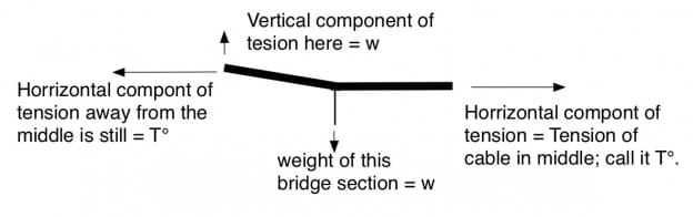
Vector diagram of forces on the cable at the center-left of the bridge.
Consider the above vector diagram (above) of forces on a section of the main cable near the center of the bridge. At the right, the center of the bridge, the cable is horizontal, and has a significant tension. Let’s call that T°. Away from the center of the bridge, there is a vertical cable supporting a fraction of roadway. Lets call the force on this point w. It equals the weight of this section of cable and this section of roadway. Because of this weight, the main cable bends upward to the left and carries more tension than T°. The tangent (slope) of the upward curve will equal w/T°, and the new tension will be the vector sum along the new slope. From geometry, T= √(w2 +T°2).

Vector diagram of forces on the cable further from the center of the bridge.
As we continue from the center, there are more and more verticals, each supporting approximately the same weight, w. From geometry, if w weight is added at each vertical, the change in slope is always w/T° as shown. When you reach the towers, the weight of the bridge must equal 2T Sin Θ, where Θ is the angle of the bridge cable at the tower and T is the tension in the cable at the tower.
The limit to the weight of a bridge, and thus its length, is the maximum tension in the main cable, T, and the maximum angle, that at the towers. Θ. I assumed that the maximum bridge would be made of T1 bridge steel, the strongest material I could think of, with a tensile strength of 100,000 psi, and I imagined a maximum angle at the towers of 30°. Since there are two towers and sin 30° = 1/2, it becomes clear that, with this 30° angle cable, the tension at the tower must equal the total weight of the bridge. Interesting.
Now, to find the length of the bridge, note that the weight of the bridge is proportional to its length times the density and cross section of the metal. I imagined a bridge where the half of the weight was in the main cable, and the rest was in the roadway, cars and verticals. If the main cable is made of T1 “bridge steel”, the density of the cable is 0.2833 lb/in3, and the density of the bridge is twice this. If the bridge cable is at its yield strength, 100,000 psi, at the towers, it must be that each square inch of cable supports 50,000 pounds of cable and 50,000 lbs of cars, roadway and verticals. The maximum length (with no allowance for wind or a safety factor) is thus
L(max) = 100,000 psi / 2 x 0.2833 pounds/in3 = 176,500 inches = 14,700 feet = 2.79 miles.
This was more than three times the length of the Verrazano bridge, whose main span is 4,260 ft. I attributed the difference to safety factors, wind, price, etc. I then set out to calculate the height of the towers, and the only rational approach I could think of involved calculus. Fortunately, I could integrate for the curve now that I knew the slope changed linearly with distance from the center. That is for every length between verticals, the slope changes by the same amount, w/T°. This was to say that d2y/dx2 = w/T° and the curve this described was a parabola.
Rather than solving with heavy calculus, I noticed that the slope, dy/dx increases in proportion to x, and since the slope at the end, at L/2, was that of a 30° triangle, 1/√3, it was clear to me that
dy/dx = (x/(L/2))/√3
where x is the distance from the center of the bridge, and L is the length of the bridge, 14,700 ft. dy/dx = 2x/L√3.
We find that:
H = ∫dy = ∫ 2x/L√3 dx = L/4√3 = 2122 ft,
where H is the height of the towers. Calculated this way, the towers were quite tall, higher than that of any building then standing, but not impossibly high (the Dubai tower is higher). It was fairly clear that you didn’t want a tower much higher than this, though, suggesting that you didn’t want to go any higher than a 30° angle for the main cable.
I decided that suspension bridges had some advantages over other designs in that they avoid the problem of beam “buckling.’ Further, they readjust their shape somewhat to accommodate heavy point loads. Arch and truss bridges don’t do this, quite. Since the towers were quite a lot taller than any building then in existence, I came to I decide that this length, 2.79 miles, was about as long as you could make the main span of a bridge.
I later came to discover materials with a higher strength per weight (titanium, fiber glass, aramid, carbon fiber…) and came to think you could go longer, but the calculation is the same, and any practical bridge would be shorter, if only because of the need for a safety factor. I also came to recalculate the height of the towers without calculus, and got an answer that was shorter, for some versions, a hundred feet shorter, as shown here. In terms of wind, I note that you could make the bridge so heavy that you don’t have to worry about wind except for resonance effects. Those are the effects are significant, but were not my concern at the moment.

The Brooklyn Bridge showing its main cable suspension structure and its catenaries.
Now to discuss catenaries, the diagonal wires that support many modern bridges and that, on the Brooklyn bridge, provide support at the ends of the spans only. Since the catenaries support some weight of the Brooklyn bridge, they decrease the need for very thick cables and very high towers. The benefit goes down as the catenary angle goes to the horizontal, though as the lower the angle the longer the catenary, and the lower the fraction of the force goes into lift. I suspect this is why Roebling used catenaries only near the Brooklyn bridge towers, for angles no more than about 45°. I was very proud of all this when I thought it through and explained it to a friend. It still gives me joy to explain it here.
Robert Buxbaum, May 16, 2019. I’ve wondered about adding vibration dampers to very long bridges to decrease resonance problems. It seems like a good idea. Though I have never gone so far as to do calculations along these lines, I note that several of the world’s tallest buildings were made of concrete, not steel, because concrete provides natural vibration damping.
 Parallel lines have so much in common.